~/data/oecd/

Info

source	dataset	.html	.RData
oecd	NRR	2024-04-15	2024-04-08

Data on wages

load_data("employment.RData")
employment %>%
  source_dataset_title_file_updates()

source	dataset	.html	.RData
bls	jt	2024-03-20	NA
bls	la	2024-01-06	NA
bls	ln	2024-01-06	NA
eurostat	nama_10_a10_e	2024-04-15	2024-04-09
eurostat	nama_10_a64_e	2024-04-15	2024-04-15
eurostat	namq_10_a10_e	2024-04-15	2024-04-15
eurostat	une_rt_m	2024-04-15	2024-04-09
oecd	ALFS_EMP	2024-04-16	2024-01-26
oecd	EPL_T	2024-04-16	2023-12-10
oecd	LFS_SEXAGE_I_R	2024-04-16	2024-04-15
oecd	STLABOUR	2024-04-15	2024-04-15

Last

obsTime	Nobs
2023	199680

Data Structure

NRR_var %>%
  pluck("VAR_DESC") %>%
  {if (is_html_output()) print_table(.) else .}

id	description
LOCATION	Country
FAMILY	Family type
DURATION	Unemployment duration (months)
EARNINGS	Previous in-work earnings
HBTOPUPS	Include housing benefits
TIME	Year
OBS_VALUE	Observation Value
TIME_FORMAT	Time Format
OBS_STATUS	Observation Status

FAMILY

NRR_var %>%
  pluck("FAMILY") %>%
  {if (is_html_output()) print_table(.) else .}

id	label
SINGLE	Single person without children
SINGLE2C	Single person with 2 children
1EARNERC	Couple without children - partner is out of work
1EARNERC2C	Couple with 2 children - partner is out of work
2EARNERC_AW	Couple without children - partner’s earnings: Average Wage (AW)
2EARNERC_67AW	Couple without children - partner’s earnings: 67% of the AW
2EARNERC2C_AW	Couple with 2 children - partner’s earnings: AW
2EARNERC2C_67AW	Couple with 2 children - partner’s earnings: 67% of the AW

DURATION

NRR_var %>%
  pluck("DURATION") %>%
  {if (is_html_output()) datatable(., filter = 'top', rownames = F) else .}

EARNINGS

NRR_var %>%
  pluck("EARNINGS") %>%
  {if (is_html_output()) print_table(.) else .}

id	label
MIN	Minimum Wage
67AW	67% of the Average Wage
AW	Average Wage

Ex 1: Average Wage

Germany

NRR %>%
  filter(LOCATION == "DEU", 
         FAMILY == "SINGLE", 
         EARNINGS == "AW", 
         HBTOPUPS == 1,
         obsTime %in% c("2001", "2005", "2018")) %>%
  mutate(DURATION = DURATION %>% as.numeric,
         obsValue = obsValue / 100) %>%
  arrange(obsTime, DURATION) %>%
  select(obsTime, DURATION, obsValue) %>%
  ggplot() + theme_minimal() +
  geom_line(aes(x = DURATION, y = obsValue, color = obsTime, linetype = obsTime)) + 
  scale_color_manual(values = viridis(4)[1:3]) +
  theme(legend.position = c(0.45, 0.9),
        legend.title = element_blank()) +
  xlab("") + ylab("Net Replacement Rate") +
  scale_x_continuous(breaks = seq(0, 60, 6),
                     labels = dollar_format(prefix = "", suffix = " mo")) +
  scale_y_continuous(breaks = seq(0, 1, 0.1),
                     labels = percent_format(accuracy = 1),
                     limits = c(0, 1))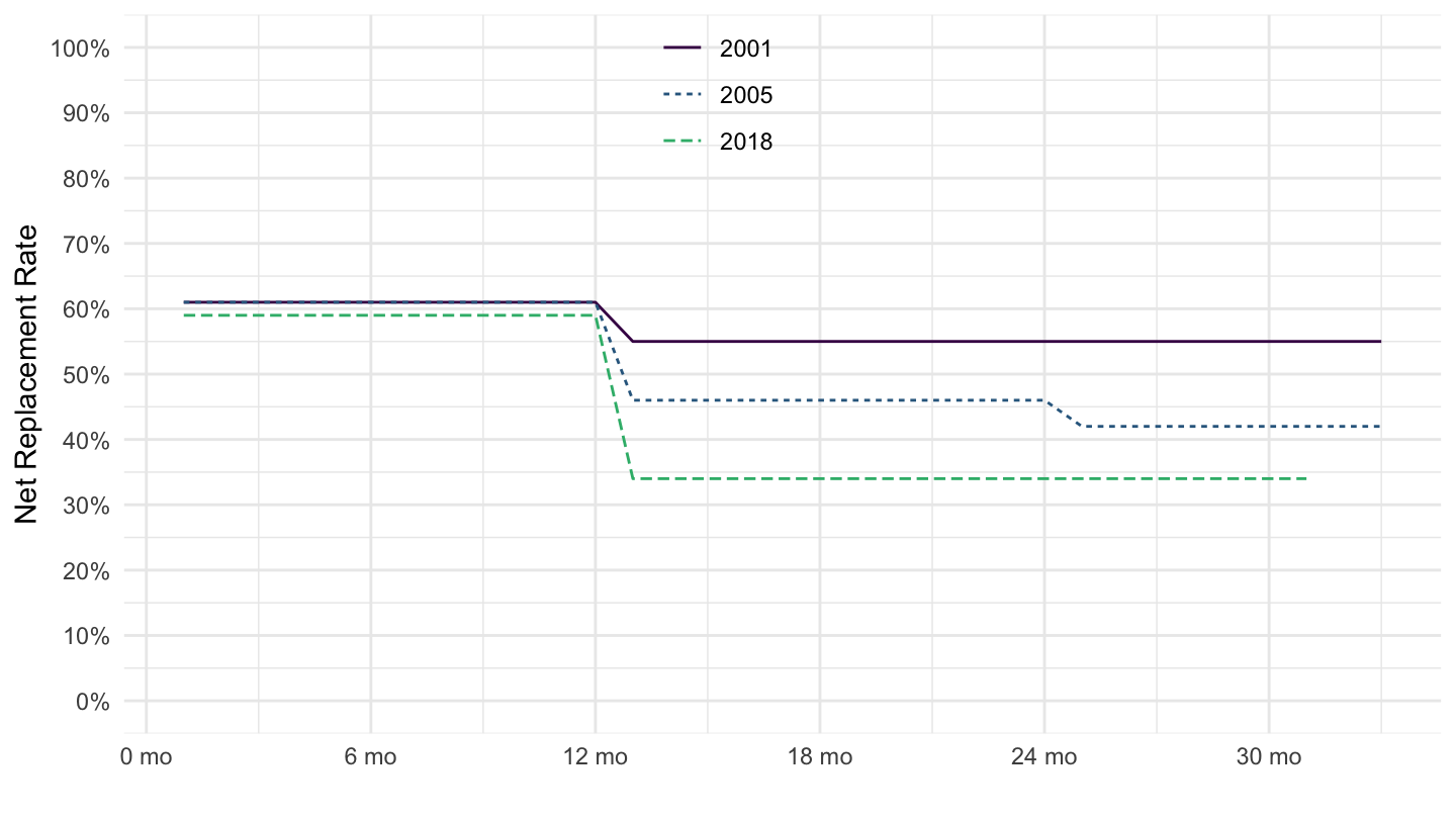

France

NRR %>%
  filter(LOCATION == "FRA", 
         FAMILY == "SINGLE", 
         EARNINGS == "AW", 
         HBTOPUPS == 1,
         obsTime %in% c("2001", "2005", "2018")) %>%
  mutate(DURATION = DURATION %>% as.numeric,
         obsValue = obsValue / 100) %>%
  arrange(obsTime, DURATION) %>%
  select(obsTime, DURATION, obsValue) %>%
  ggplot() + theme_minimal() +
  geom_line(aes(x = DURATION, y = obsValue, color = obsTime, linetype = obsTime)) + 
  scale_color_manual(values = viridis(4)[1:3]) +
  theme(legend.position = c(0.85, 0.9),
        legend.title = element_blank()) +
  xlab("") + ylab("Net Replacement Rate") +
  scale_x_continuous(breaks = seq(0, 60, 6),
                     labels = dollar_format(prefix = "", suffix = " mo")) +
  scale_y_continuous(breaks = seq(0, 1, 0.1),
                     labels = percent_format(accuracy = 1),
                     limits = c(0, 1))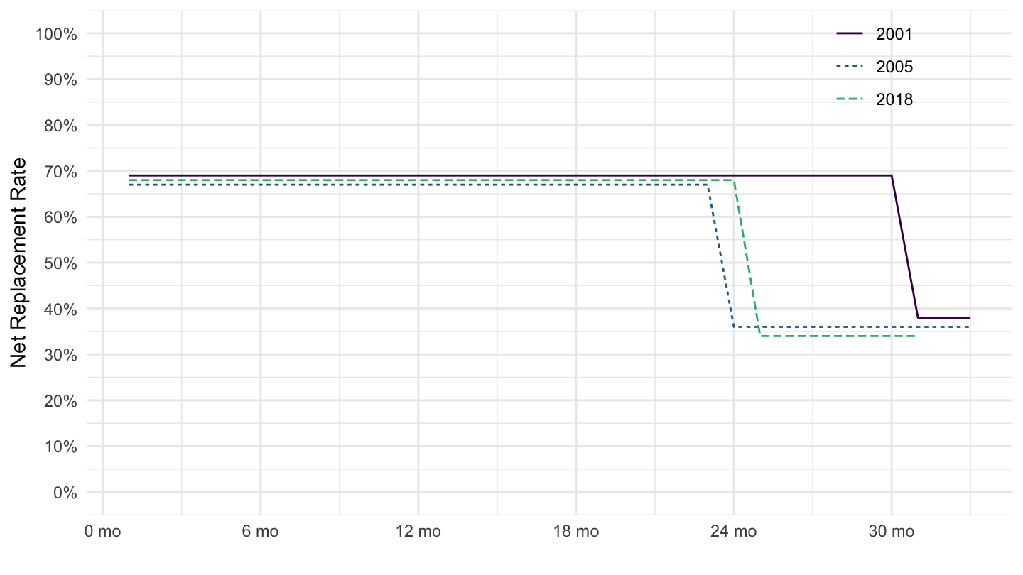

Italy

NRR %>%
  filter(LOCATION == "ITA", 
         FAMILY == "SINGLE", 
         EARNINGS == "AW", 
         HBTOPUPS == 1,
         obsTime %in% c("2001", "2005", "2018")) %>%
  mutate(DURATION = DURATION %>% as.numeric,
         obsValue = obsValue / 100) %>%
  arrange(obsTime, DURATION) %>%
  select(obsTime, DURATION, obsValue) %>%
  ggplot() + theme_minimal() +
  geom_line(aes(x = DURATION, y = obsValue, color = obsTime, linetype = obsTime)) + 
  scale_color_manual(values = viridis(4)[1:3]) +
  theme(legend.position = c(0.85, 0.9),
        legend.title = element_blank()) +
  xlab("") + ylab("Net Replacement Rate") +
  scale_x_continuous(breaks = seq(0, 60, 6),
                     labels = dollar_format(prefix = "", suffix = " mo")) +
  scale_y_continuous(breaks = seq(0, 1, 0.1),
                     labels = percent_format(accuracy = 1),
                     limits = c(0, 1))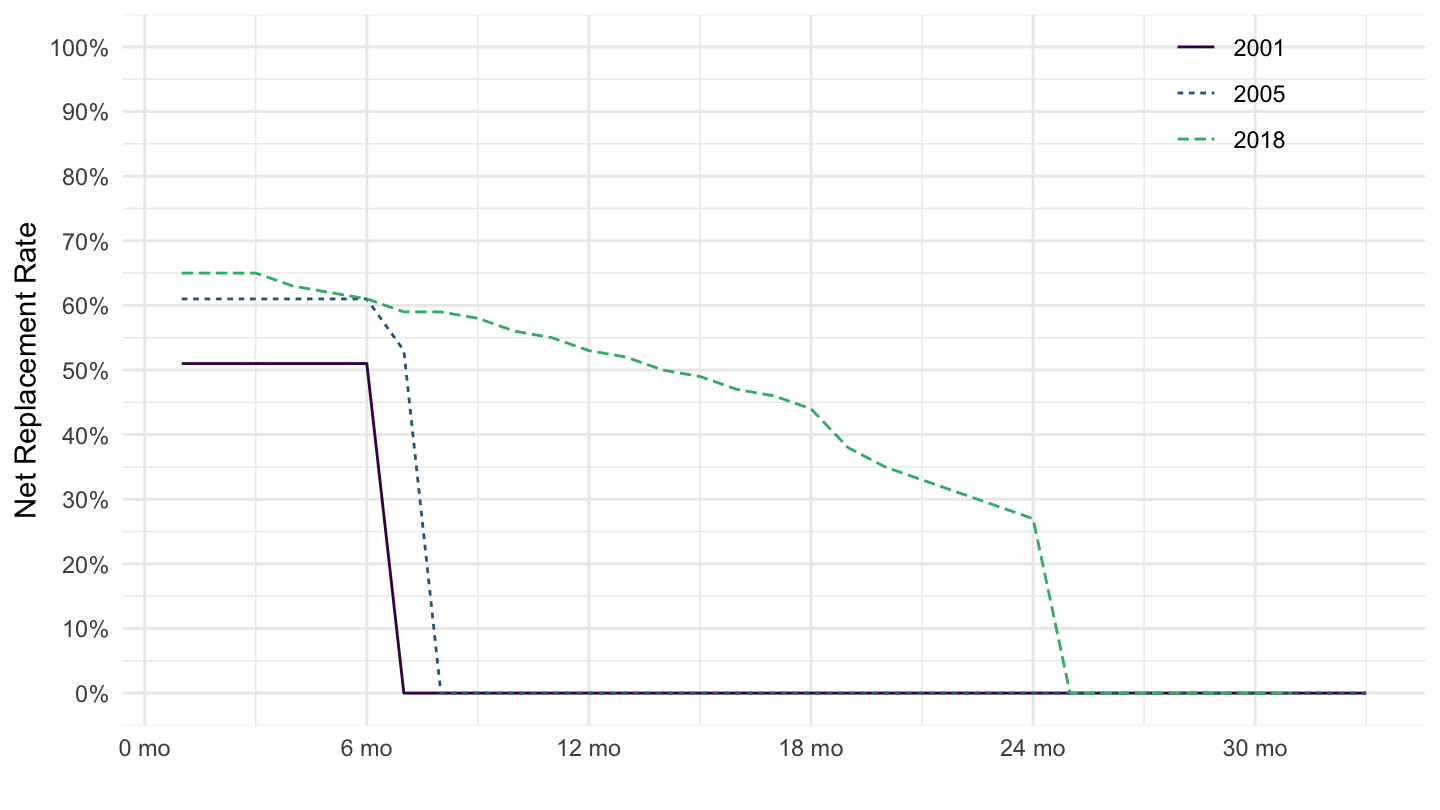

Spain

NRR %>%
  filter(LOCATION == "ESP", 
         FAMILY == "SINGLE", 
         EARNINGS == "AW", 
         HBTOPUPS == 1,
         obsTime %in% c("2001", "2005", "2018")) %>%
  mutate(DURATION = DURATION %>% as.numeric,
         obsValue = obsValue / 100) %>%
  arrange(obsTime, DURATION) %>%
  select(obsTime, DURATION, obsValue) %>%
  ggplot() + theme_minimal() +
  geom_line(aes(x = DURATION, y = obsValue, color = obsTime, linetype = obsTime)) + 
  scale_color_manual(values = viridis(4)[1:3]) +
  theme(legend.position = c(0.85, 0.9),
        legend.title = element_blank()) +
  xlab("") + ylab("Net Replacement Rate") +
  scale_x_continuous(breaks = seq(0, 60, 6),
                     labels = dollar_format(prefix = "", suffix = " mo")) +
  scale_y_continuous(breaks = seq(0, 1, 0.1),
                     labels = percent_format(accuracy = 1),
                     limits = c(0, 1))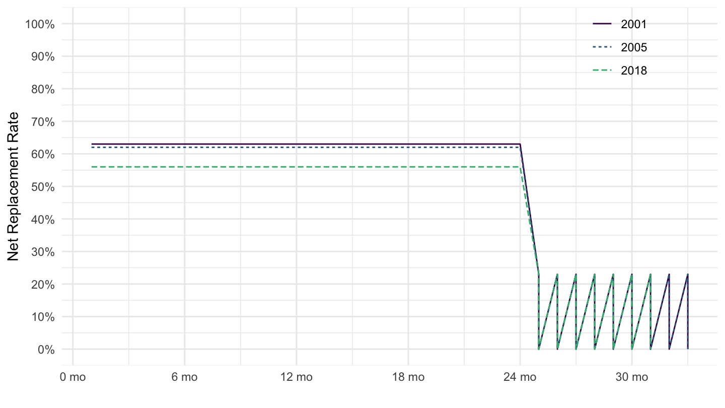

United Kingdom

NRR %>%
  filter(LOCATION == "GBR", 
         FAMILY == "SINGLE", 
         EARNINGS == "AW", 
         HBTOPUPS == 1,
         obsTime %in% c("2001", "2005", "2018")) %>%
  mutate(DURATION = DURATION %>% as.numeric,
         obsValue = obsValue / 100) %>%
  arrange(obsTime, DURATION) %>%
  select(obsTime, DURATION, obsValue) %>%
  ggplot() + theme_minimal() +
  geom_line(aes(x = DURATION, y = obsValue, color = obsTime, linetype = obsTime)) + 
  scale_color_manual(values = viridis(4)[1:3]) +
  theme(legend.position = c(0.85, 0.9),
        legend.title = element_blank()) +
  xlab("") + ylab("Net Replacement Rate") +
  scale_x_continuous(breaks = seq(0, 60, 6),
                     labels = dollar_format(prefix = "", suffix = " mo")) +
  scale_y_continuous(breaks = seq(0, 1, 0.1),
                     labels = percent_format(accuracy = 1),
                     limits = c(0, 1))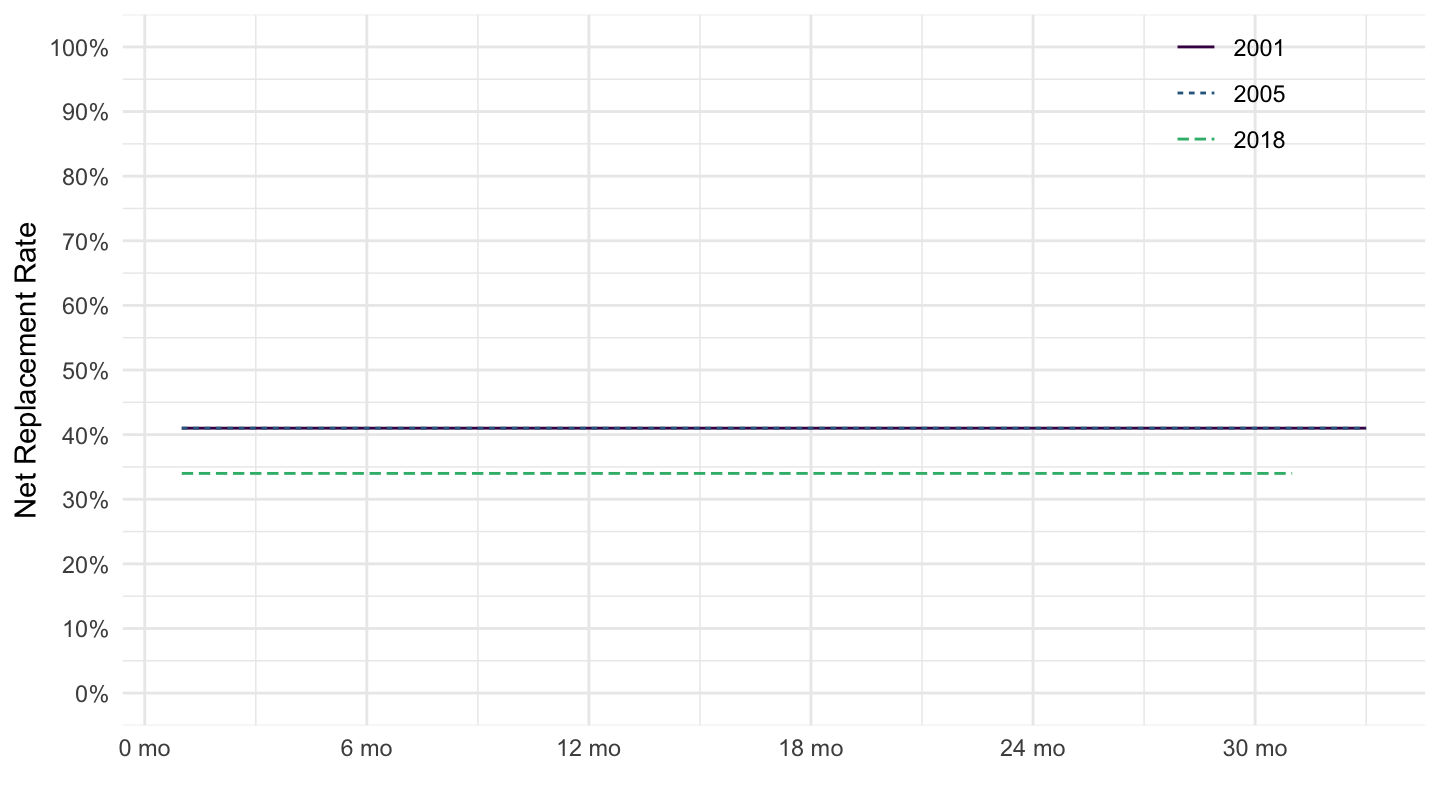

United States

NRR %>%
  filter(LOCATION == "USA", 
         FAMILY == "SINGLE", 
         EARNINGS == "AW", 
         HBTOPUPS == 1,
         obsTime %in% c("2001", "2005", "2018")) %>%
  mutate(DURATION = DURATION %>% as.numeric,
         obsValue = obsValue / 100) %>%
  arrange(obsTime, DURATION) %>%
  select(obsTime, DURATION, obsValue) %>%
  ggplot() + theme_minimal() +
  geom_line(aes(x = DURATION, y = obsValue, color = obsTime, linetype = obsTime)) + 
  scale_color_manual(values = viridis(4)[1:3]) +
  theme(legend.position = c(0.85, 0.9),
        legend.title = element_blank()) +
  xlab("") + ylab("Net Replacement Rate") +
  scale_x_continuous(breaks = seq(0, 60, 6),
                     labels = dollar_format(prefix = "", suffix = " mo")) +
  scale_y_continuous(breaks = seq(0, 1, 0.1),
                     labels = percent_format(accuracy = 1),
                     limits = c(0, 1))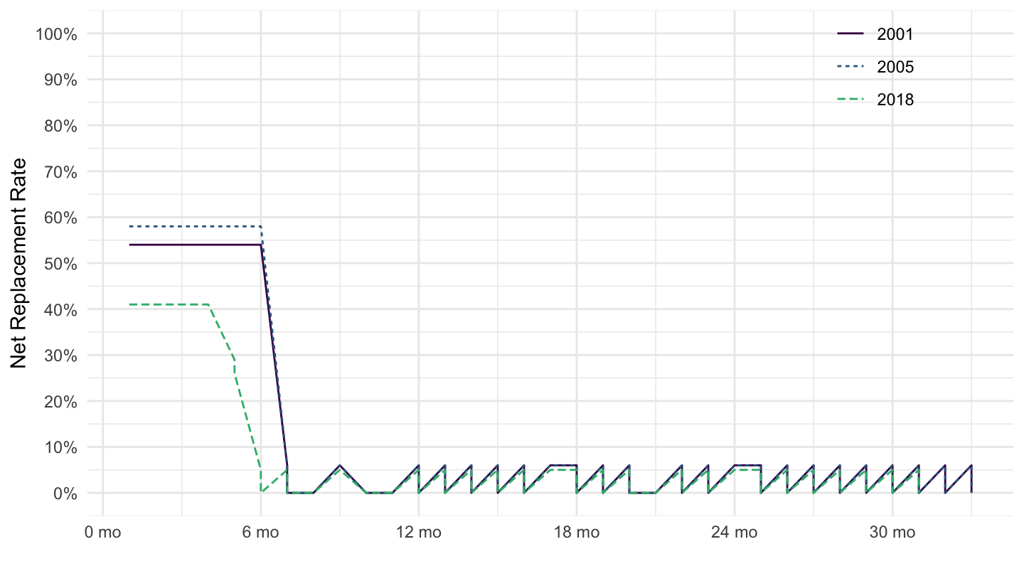

Switzerland

NRR %>%
  filter(LOCATION == "CHE", 
         FAMILY == "SINGLE", 
         EARNINGS == "AW", 
         HBTOPUPS == 1,
         obsTime %in% c("2001", "2005", "2018")) %>%
  mutate(DURATION = DURATION %>% as.numeric,
         obsValue = obsValue / 100) %>%
  arrange(obsTime, DURATION) %>%
  select(obsTime, DURATION, obsValue) %>%
  ggplot() + theme_minimal() +
  geom_line(aes(x = DURATION, y = obsValue, color = obsTime, linetype = obsTime)) + 
  scale_color_manual(values = viridis(4)[1:3]) +
  theme(legend.position = c(0.85, 0.9),
        legend.title = element_blank()) +
  xlab("") + ylab("Net Replacement Rate") +
  scale_x_continuous(breaks = seq(0, 60, 6),
                     labels = dollar_format(prefix = "", suffix = " mo")) +
  scale_y_continuous(breaks = seq(0, 1, 0.1),
                     labels = percent_format(accuracy = 1),
                     limits = c(0, 1))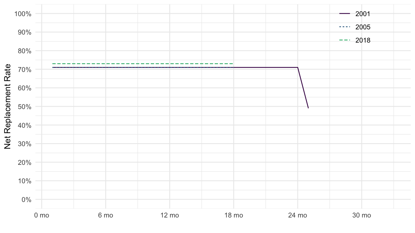

Ex 2: Minimum Wage

Germany

NRR %>%
  filter(LOCATION == "DEU", 
         FAMILY == "SINGLE", 
         EARNINGS == "MIN", 
         HBTOPUPS == 1,
         obsTime %in% c("2001", "2005", "2018")) %>%
  mutate(DURATION = DURATION %>% as.numeric,
         obsValue = obsValue / 100) %>%
  arrange(obsTime, DURATION) %>%
  select(obsTime, DURATION, obsValue) %>%
  ggplot() + theme_minimal() +
  geom_line(aes(x = DURATION, y = obsValue, color = obsTime, linetype = obsTime)) + 
  scale_color_manual(values = viridis(4)[1:3]) +
  theme(legend.position = c(0.45, 0.9),
        legend.title = element_blank()) +
  xlab("") + ylab("Net Replacement Rate") +
  scale_x_continuous(breaks = seq(0, 60, 6),
                     labels = dollar_format(prefix = "", suffix = " mo")) +
  scale_y_continuous(breaks = seq(0, 1, 0.1),
                     labels = percent_format(accuracy = 1),
                     limits = c(0, 1))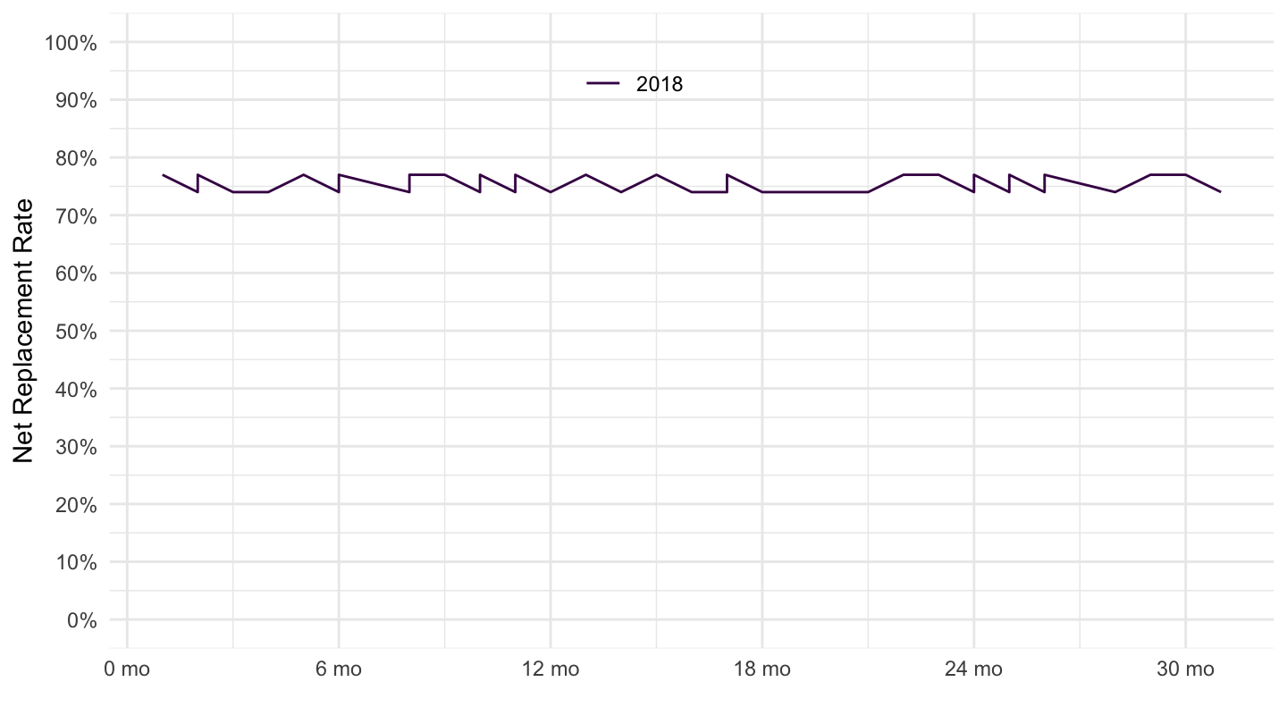

France

NRR %>%
  filter(LOCATION == "FRA", 
         FAMILY == "SINGLE", 
         EARNINGS == "MIN", 
         HBTOPUPS == 1,
         obsTime %in% c("2001", "2005", "2018")) %>%
  mutate(DURATION = DURATION %>% as.numeric,
         obsValue = obsValue / 100) %>%
  arrange(obsTime, DURATION) %>%
  select(obsTime, DURATION, obsValue) %>%
  ggplot() + theme_minimal() +
  geom_line(aes(x = DURATION, y = obsValue, color = obsTime, linetype = obsTime)) + 
  scale_color_manual(values = viridis(4)[1:3]) +
  theme(legend.position = c(0.85, 0.9),
        legend.title = element_blank()) +
  xlab("") + ylab("Net Replacement Rate") +
  scale_x_continuous(breaks = seq(0, 60, 6),
                     labels = dollar_format(prefix = "", suffix = " mo")) +
  scale_y_continuous(breaks = seq(0, 1, 0.1),
                     labels = percent_format(accuracy = 1),
                     limits = c(0, 1))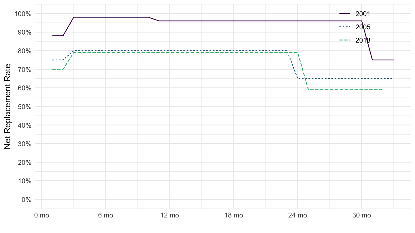

Italy

NRR %>%
  filter(LOCATION == "ITA", 
         FAMILY == "SINGLE", 
         EARNINGS == "MIN", 
         HBTOPUPS == 1,
         obsTime %in% c("2001", "2005", "2018")) %>%
  mutate(DURATION = DURATION %>% as.numeric,
         obsValue = obsValue / 100) %>%
  arrange(obsTime, DURATION) %>%
  select(obsTime, DURATION, obsValue) %>%
  ggplot() + theme_minimal() +
  geom_line(aes(x = DURATION, y = obsValue, color = obsTime, linetype = obsTime)) + 
  scale_color_manual(values = viridis(4)[1:3]) +
  theme(legend.position = c(0.85, 0.9),
        legend.title = element_blank()) +
  xlab("") + ylab("Net Replacement Rate") +
  scale_x_continuous(breaks = seq(0, 60, 6),
                     labels = dollar_format(prefix = "", suffix = " mo")) +
  scale_y_continuous(breaks = seq(0, 1, 0.1),
                     labels = percent_format(accuracy = 1),
                     limits = c(0, 1))

Spain

NRR %>%
  filter(LOCATION == "ESP", 
         FAMILY == "SINGLE", 
         EARNINGS == "MIN", 
         HBTOPUPS == 1,
         obsTime %in% c("2001", "2005", "2018")) %>%
  mutate(DURATION = DURATION %>% as.numeric,
         obsValue = obsValue / 100) %>%
  arrange(obsTime, DURATION) %>%
  select(obsTime, DURATION, obsValue) %>%
  ggplot() + theme_minimal() +
  geom_line(aes(x = DURATION, y = obsValue, color = obsTime, linetype = obsTime)) + 
  scale_color_manual(values = viridis(4)[1:3]) +
  theme(legend.position = c(0.85, 0.9),
        legend.title = element_blank()) +
  xlab("") + ylab("Net Replacement Rate") +
  scale_x_continuous(breaks = seq(0, 60, 6),
                     labels = dollar_format(prefix = "", suffix = " mo")) +
  scale_y_continuous(breaks = seq(0, 1, 0.1),
                     labels = percent_format(accuracy = 1),
                     limits = c(0, 1))

United Kingdom

NRR %>%
  filter(LOCATION == "GBR", 
         FAMILY == "SINGLE", 
         EARNINGS == "MIN", 
         HBTOPUPS == 1,
         obsTime %in% c("2001", "2005", "2018")) %>%
  mutate(DURATION = DURATION %>% as.numeric,
         obsValue = obsValue / 100) %>%
  arrange(obsTime, DURATION) %>%
  select(obsTime, DURATION, obsValue) %>%
  ggplot() + theme_minimal() +
  geom_line(aes(x = DURATION, y = obsValue, color = obsTime, linetype = obsTime)) + 
  scale_color_manual(values = viridis(4)[1:3]) +
  theme(legend.position = c(0.85, 0.9),
        legend.title = element_blank()) +
  xlab("") + ylab("Net Replacement Rate") +
  scale_x_continuous(breaks = seq(0, 60, 6),
                     labels = dollar_format(prefix = "", suffix = " mo")) +
  scale_y_continuous(breaks = seq(0, 1, 0.1),
                     labels = percent_format(accuracy = 1),
                     limits = c(0, 1))

United States

NRR %>%
  filter(LOCATION == "USA", 
         FAMILY == "SINGLE", 
         EARNINGS == "MIN", 
         HBTOPUPS == 1,
         obsTime %in% c("2001", "2005", "2018")) %>%
  mutate(DURATION = DURATION %>% as.numeric,
         obsValue = obsValue / 100) %>%
  arrange(obsTime, DURATION) %>%
  select(obsTime, DURATION, obsValue) %>%
  ggplot() + theme_minimal() +
  geom_line(aes(x = DURATION, y = obsValue, color = obsTime, linetype = obsTime)) + 
  scale_color_manual(values = viridis(4)[1:3]) +
  theme(legend.position = c(0.85, 0.9),
        legend.title = element_blank()) +
  xlab("") + ylab("Net Replacement Rate") +
  scale_x_continuous(breaks = seq(0, 60, 6),
                     labels = dollar_format(prefix = "", suffix = " mo")) +
  scale_y_continuous(breaks = seq(0, 1, 0.1),
                     labels = percent_format(accuracy = 1),
                     limits = c(0, 1))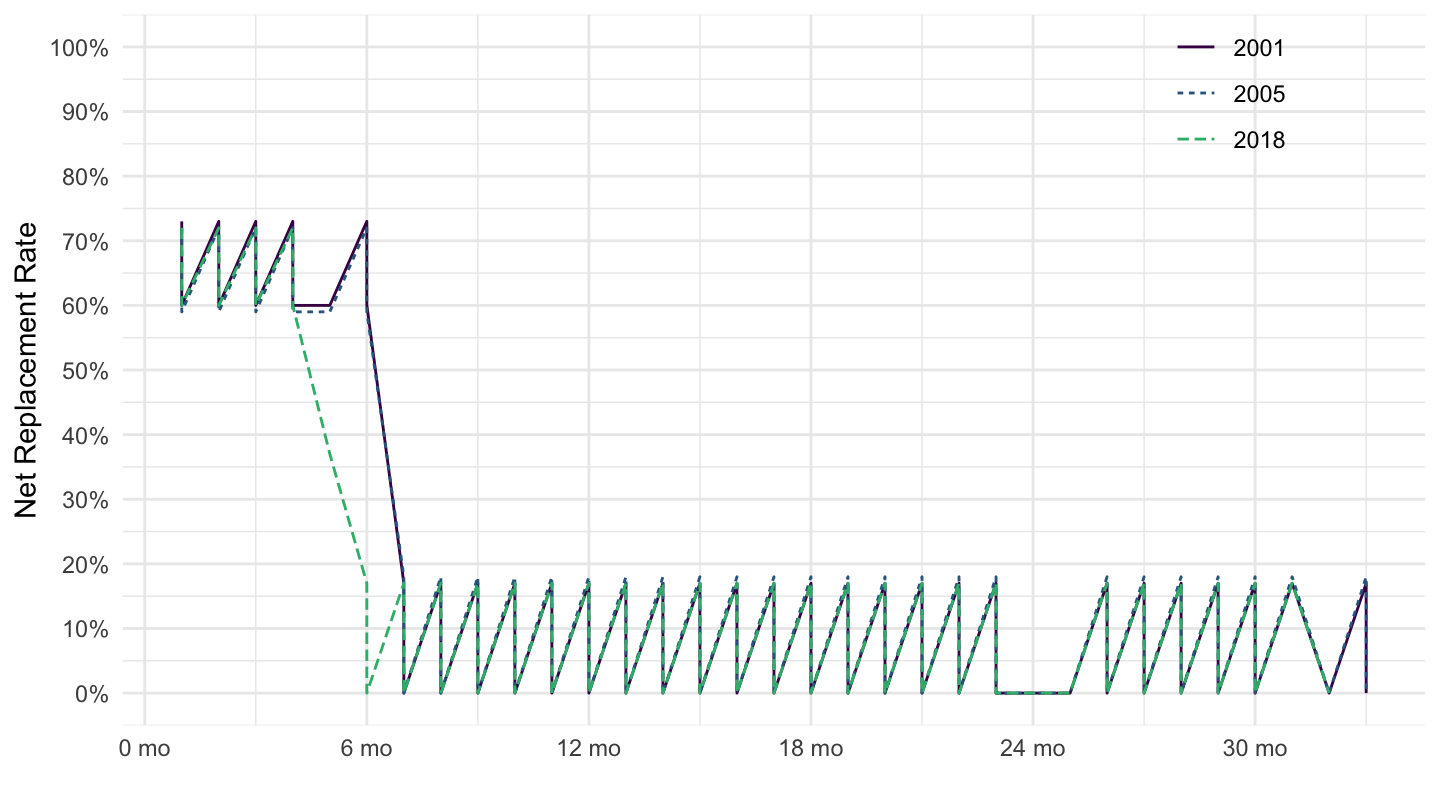

Switzerland

NRR %>%
  filter(LOCATION == "CHE", 
         FAMILY == "SINGLE", 
         EARNINGS == "MIN", 
         HBTOPUPS == 1,
         obsTime %in% c("2001", "2005", "2018")) %>%
  mutate(DURATION = DURATION %>% as.numeric,
         obsValue = obsValue / 100) %>%
  arrange(obsTime, DURATION) %>%
  select(obsTime, DURATION, obsValue) %>%
  ggplot() + theme_minimal() +
  geom_line(aes(x = DURATION, y = obsValue, color = obsTime, linetype = obsTime)) + 
  scale_color_manual(values = viridis(4)[1:3]) +
  theme(legend.position = c(0.85, 0.9),
        legend.title = element_blank()) +
  xlab("") + ylab("Net Replacement Rate") +
  scale_x_continuous(breaks = seq(0, 60, 6),
                     labels = dollar_format(prefix = "", suffix = " mo")) +
  scale_y_continuous(breaks = seq(0, 1, 0.1),
                     labels = percent_format(accuracy = 1),
                     limits = c(0, 1))

Net Replacement Rates in unemployment - NRR

Data - OECD

François Geerolf

Info

Data on wages

Last

Data Structure

FAMILY

DURATION

EARNINGS

Ex 1: Average Wage

Germany

France

Italy

Spain

United Kingdom

United States

Switzerland

Ex 2: Minimum Wage

Germany

France

Italy

Spain

United Kingdom

United States

Switzerland