
Last observation: Q2 2026 (N = 70)
First observation: Q1 1949 (N = 70)
Last data update: 03 sept. 2026, 05:31
Last compile: 10 oct. 2026, 02:00
Récapitulatif trimestriel des comptes de production et d’exploitation par branche (prix courants). Les libellés de branche sont reconstitués à partir de l’en-tête du fichier source.
| Opération | Nobs |
|---|---|
| Consommation intermédiaire des branches | 7130 |
| Production branche | 7440 |
| Valeur ajoutée brute des branches | 7130 |
RB |>
  filter(operation == "Valeur ajoutée brute des branches", code %in% gsub("P1E_", "B1_", b17)) |>
  group_by(date) |> mutate(part = value / sum(value)) |> ungroup() |>
  arrange(desc(code)) |> mutate(poste = factor(poste, levels = unique(poste))) |>
  ggplot() + theme_minimal() + xlab("") + ylab("Part de la valeur ajoutée") +
  geom_area(aes(x = date, y = part, fill = poste)) +
  scale_x_date(date_breaks = "10 years", date_labels = "%Y") +
  scale_y_continuous(labels = percent_format(accuracy = 1)) +
  scale_fill_viridis_d() +
  theme(legend.title = element_blank(), legend.position = "bottom",
        legend.text = element_text(size = 6.5)) +
  guides(fill = guide_legend(ncol = 3))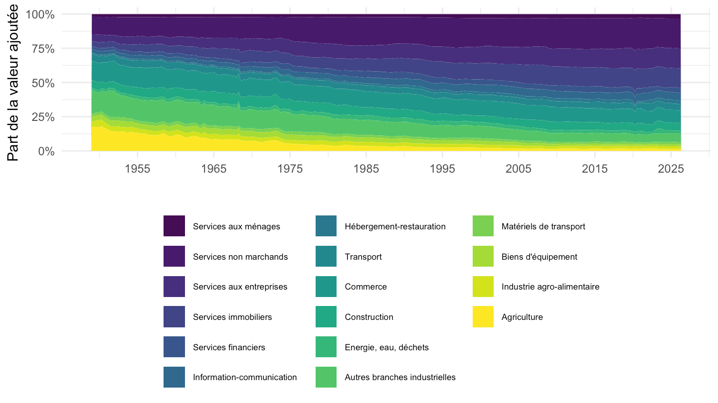
RB |>
  filter(code %in% c("P1E_DI", "P1E_DS", "P1E_FZ", "P2E_DI", "P2E_DS", "P2E_FZ")) |>
  mutate(g = sub("^P[12]E_", "", code), op = substr(code, 1, 3)) |>
  select(date, g, op, value) |>
  tidyr::pivot_wider(names_from = op, values_from = value) |>
  mutate(branche = recode(g, DI = "Industrie", DS = "Services", FZ = "Construction")) |>
  ggplot() + theme_minimal() + xlab("") + ylab("Consommations intermédiaires / production") +
  geom_line(aes(x = date, y = P2E / P1E, color = branche)) +
  scale_x_date(date_breaks = "10 years", date_labels = "%Y") +
  scale_y_continuous(labels = percent_format(accuracy = 1)) +
  theme(legend.title = element_blank(), legend.position = "bottom")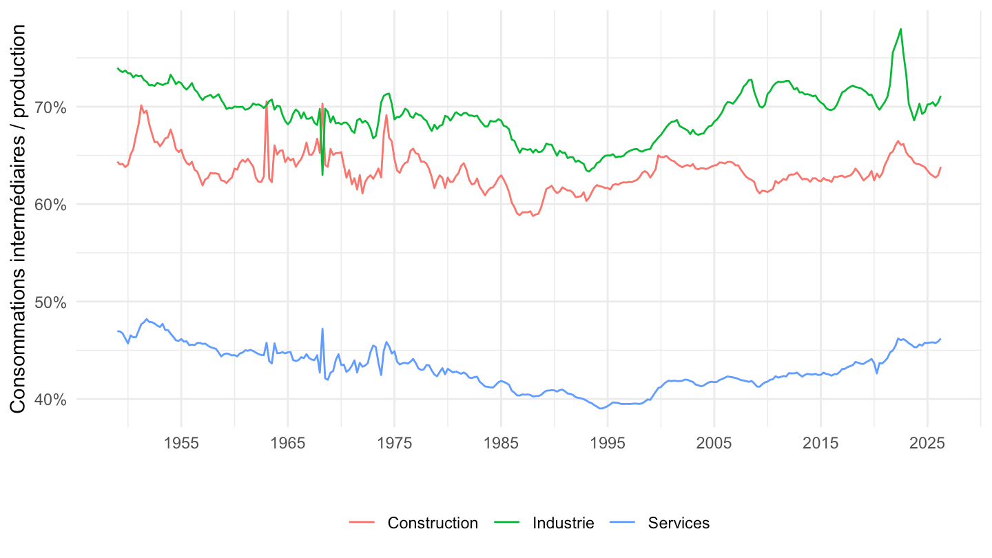
RB |>
  filter(operation == "Valeur ajoutée brute des branches",
         code %in% c("B1_D", "B1_DIM", "B1_DS")) |>
  arrange(date) |> group_by(code) |> mutate(g = value / lag(value, 4) - 1) |> ungroup() |>
  filter(date >= as.Date("1980-01-01")) |>
  mutate(branche = recode(code, B1_D = "Total", B1_DIM = "Industrie manuf.", B1_DS = "Services")) |>
  ggplot() + theme_minimal() + xlab("") + ylab("Glissement annuel de la VA") +
  geom_hline(yintercept = 0, color = "grey60") +
  geom_line(aes(x = date, y = g, color = branche)) +
  scale_x_date(date_breaks = "10 years", date_labels = "%Y") +
  scale_y_continuous(labels = percent_format(accuracy = 1)) +
  theme(legend.title = element_blank(), legend.position = "bottom")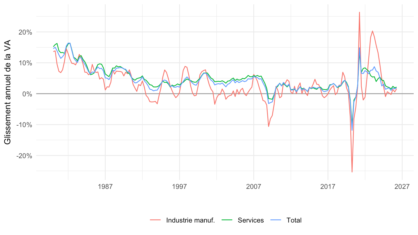
RB |>
  filter(date >= last_d %m-% months(12)) |>
  transmute(Trimestre = format(date), Opération = operation, Branche = poste,
            Valeur = round(value, 1)) %>%
  {if (is_html_output()) datatable(., filter = "top", rownames = F) else head(., 60)}