| source | dataset | Title | .html | .rData |
|---|---|---|---|---|
| insee | t_compteapu_val | Dépenses, recettes et besoin de financement des administrations publiques - valeurs aux prix courants | 2026-07-24 | 2026-02-27 |
| insee | T_7301 | 7.301 – Compte des administrations publiques (S13) (En milliards d'euros) | 2026-07-24 | 2025-10-24 |
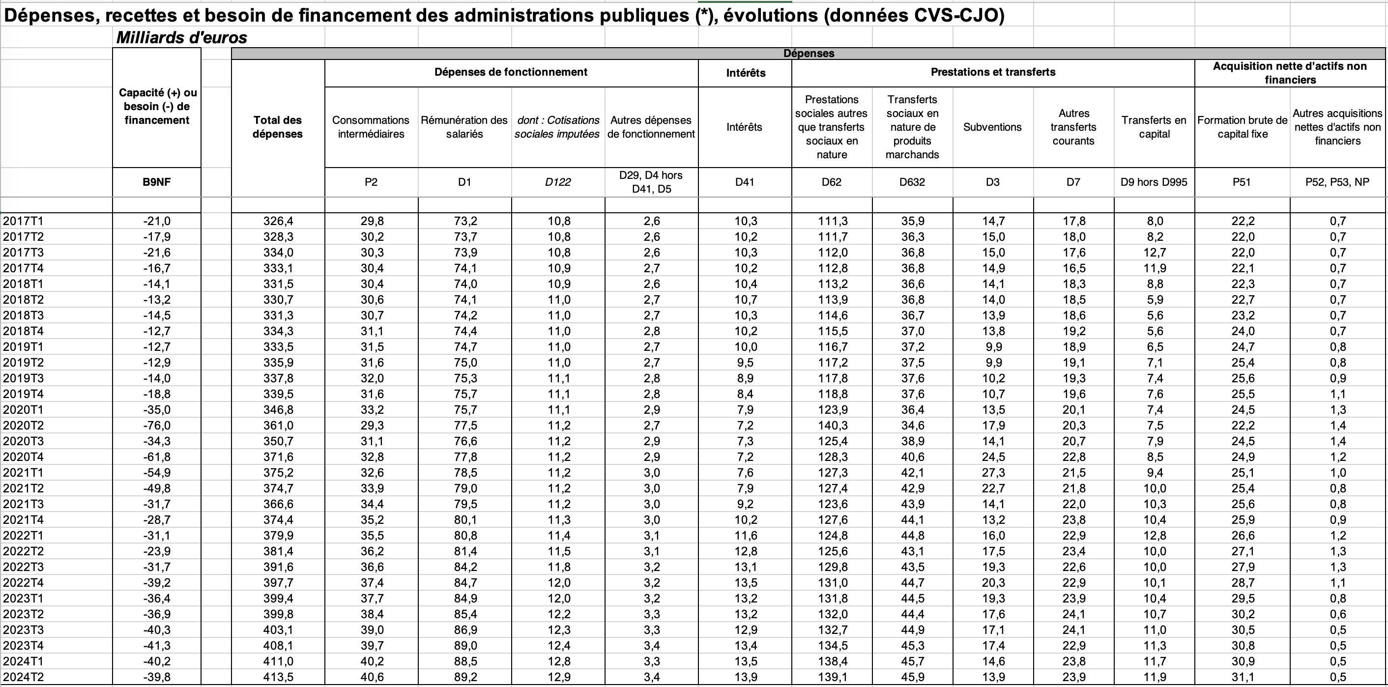
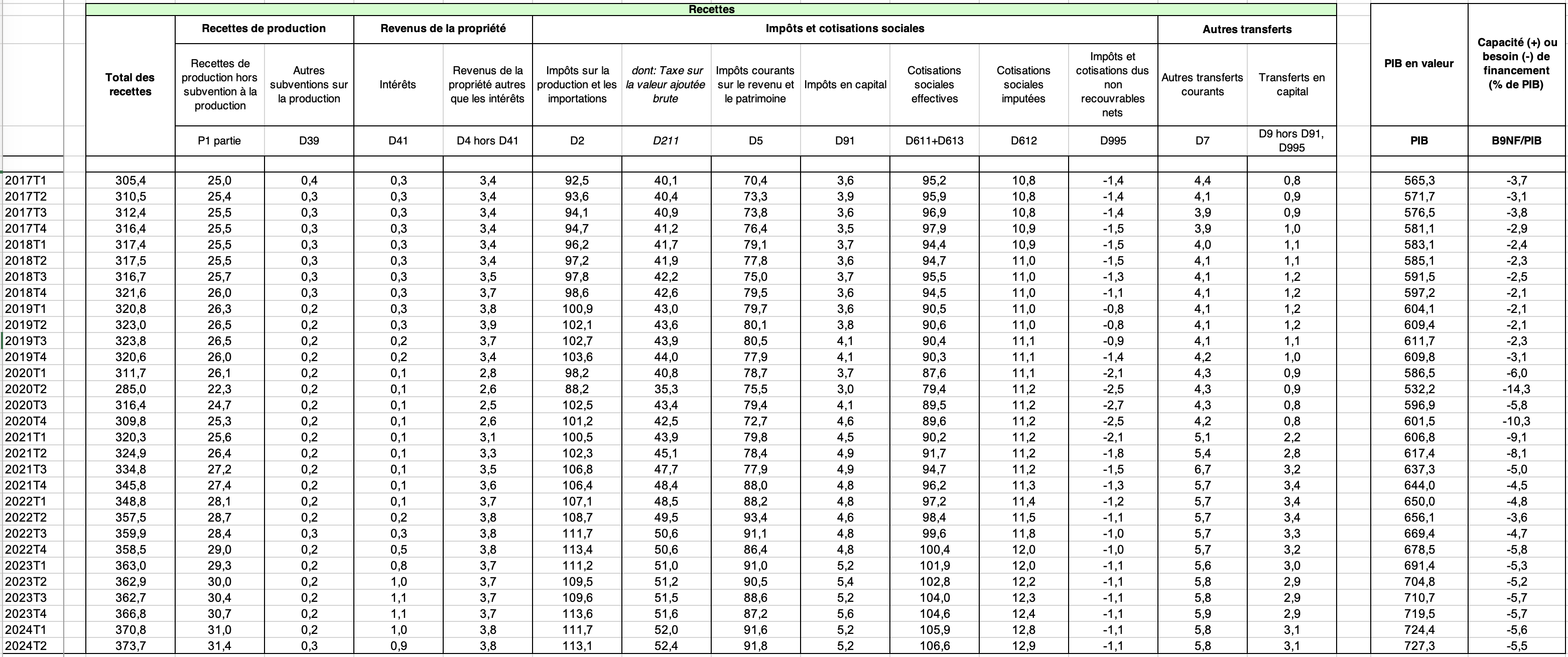
Dépenses, recettes et besoin de financement des administrations publiques - valeurs aux prix courants
Données - INSEE
Info
Données sur la dette publique
| source | dataset | Title | .html | .rData |
|---|---|---|---|---|
| gfd | debt | Debt | 2021-08-22 | 2021-03-01 |
| imf | HPDD | NA | NA | NA |
| insee | CNA-2014-DETTE-APU | Dette et déficit des administrations publiques au sens de Maastricht | 2026-07-24 | 2026-07-24 |
| insee | COMPTES-ETAT | Budget de l’État | 2026-07-24 | 2026-07-24 |
| insee | DETTE-TRIM-APU-2020 | Dette des administrations publiques au sens de Maastricht | 2026-07-24 | 2026-07-24 |
| insee | T_3217 | 3.217 – Principaux impôts par catégorie (En milliards d'euros) | 2026-07-24 | 2026-07-19 |
| insee | T_7301 | 7.301 – Compte des administrations publiques (S13) (En milliards d'euros) | 2026-07-24 | 2025-10-24 |
| insee | t_compteapu_val | Dépenses, recettes et besoin de financement des administrations publiques - valeurs aux prix courants | 2026-07-24 | 2026-02-27 |
LAST_COMPILE
| LAST_COMPILE |
|---|
| 2026-07-26 |
Last
| date | Nobs |
|---|---|
| 2025-07-01 | 30 |
Structure
column
Code
t_compteapu_val %>%
  left_join(variable, by = "column") %>%
  group_by(column, operation, Line1, Line2, Operation) %>%
  summarise(Nobs = n()) %>%
print_table_conditional()| column | operation | Line1 | Line2 | Operation | Nobs |
|---|---|---|---|---|---|
| 2 | B9NF | Capacité (+) ou besoin (-) de financement | Capacité (+) ou besoin (-) de financement | Capacité (+) ou besoin (-) de financement | 307 |
| 4 | DEPENSES | Dépenses | Dépenses | Dépenses | 183 |
| 5 | P2 | Dépenses | Dépenses de fonctionnement | Consommations intermédiaires | 307 |
| 6 | D1 | Dépenses | Dépenses de fonctionnement | Rémunération des salariés | 307 |
| 7 | D122 | Dépenses | Dépenses de fonctionnement | dont : Cotisations sociales imputées | 307 |
| 8 | D29, D4 hors D41, D5 | Dépenses | Dépenses de fonctionnement | Autres dépenses de fonctionnement | 307 |
| 9 | D41 | Dépenses | Intérêts | Intérêts | 307 |
| 10 | D62 | Dépenses | Prestations et transferts | Prestations sociales autres que transferts sociaux en nature | 307 |
| 11 | D632 | Dépenses | Prestations et transferts | Transferts sociaux en nature de produits marchands | 307 |
| 12 | D3 | Dépenses | Prestations et transferts | Subventions | 183 |
| 13 | D7 | Dépenses | Prestations et transferts | Autres transferts courants | 307 |
| 14 | D9 hors D995 | Dépenses | Prestations et transferts | Transferts en capital | 307 |
| 15 | P51 | Dépenses | Acquisition nette d'actifs non financiers | Formation brute de capital fixe | 307 |
| 16 | P52, P53, NP | Dépenses | Acquisition nette d'actifs non financiers | Autres acquisitions nettes d'actifs non financiers | 183 |
| 18 | RECETTES | Recettes | Recettes | Recettes | 183 |
| 19 | P1 partie | Recettes | Recettes de production | Recettes de production hors subvention à la production | 183 |
| 20 | D39 | Recettes | Recettes de production | Autres subventions sur la production | 183 |
| 21 | D41 | Recettes | Revenus de la propriété | Intérêts | 307 |
| 22 | D4 hors D41 | Recettes | Revenus de la propriété | Revenus de la propriété autres que les intérêts | 307 |
| 23 | D2 | Recettes | Impôts et cotisations sociales | Impôts sur la production et les importations | 307 |
| 24 | D211 | Recettes | Impôts et cotisations sociales | dont: Taxe sur la valeur ajoutée brute | 307 |
| 25 | D5 | Recettes | Impôts et cotisations sociales | Impôts courants sur le revenu et le patrimoine | 307 |
| 26 | D91 | Recettes | Impôts et cotisations sociales | Impôts en capital | 307 |
| 27 | D611+D613 | Recettes | Impôts et cotisations sociales | Cotisations sociales effectives | 307 |
| 28 | D612 | Recettes | Impôts et cotisations sociales | Cotisations sociales imputées | 307 |
| 29 | D995 | Recettes | Impôts et cotisations sociales | Impôts et cotisations dus non recouvrables nets | 191 |
| 30 | D7 | Recettes | Autres transferts | Autres transferts courants | 307 |
| 31 | D9 hors D91, D995 | Recettes | Autres transferts | Transferts en capital | 183 |
| 33 | PIB | PIB en valeur | PIB en valeur | PIB en valeur | 307 |
| 34 | B9NF/PIB | Capacité (+) ou besoin (-) de financement (% de PIB) | Capacité (+) ou besoin (-) de financement (% de PIB) | Capacité (+) ou besoin (-) de financement (% de PIB) | 307 |
Intérêts (% du PIB)
Tous
Code
t_compteapu_val %>%
  filter(column %in% c(21, 9, 33)) %>%
  spread(column, value) %>%
  transmute(date,
         `Intérêts (dépenses)` = `9`/`33`,
         `Intérêts (recettes)` = `21`/`33`) %>%
  gather(variable, value, -date) %>%
  filter(!is.na(value)) %>%
  ggplot(.) + theme_minimal() + ylab("% du PIB") + xlab("") +
  geom_line(aes(x = date, y = value, color = variable)) +
  theme(legend.title = element_blank(),
        legend.position = c(0.15, 0.9)) +
  scale_x_date(breaks = seq(1950, 2100, 5) %>% paste0("-01-01") %>% as.Date,
               labels = date_format("%Y")) +
  scale_y_continuous(breaks = 0.01*seq(0, 100, .5),
                     labels = scales::percent_format(accuracy = .1))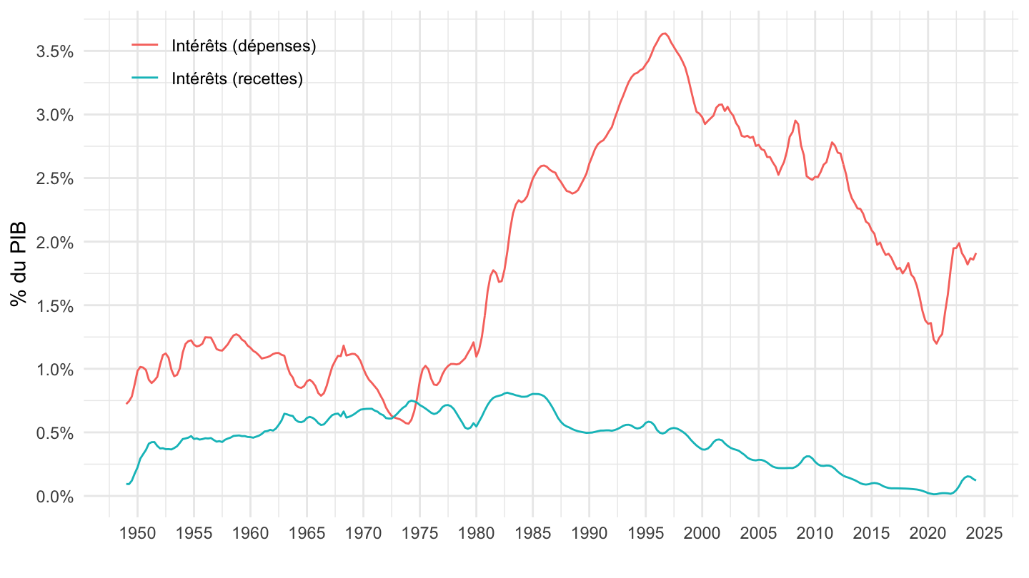
1990-
Code
t_compteapu_val %>%
  filter(column %in% c(21, 9, 33),
         date >= as.Date("1990-01-01")) %>%
  spread(column, value) %>%
  transmute(date,
         `Intérêts (dépenses)` = `9`/`33`,
         `Intérêts (recettes)` = `21`/`33`) %>%
  gather(variable, value, -date) %>%
  filter(!is.na(value)) %>%
  ggplot(.) + theme_minimal() + ylab("% du PIB") + xlab("") +
  geom_line(aes(x = date, y = value, color = variable)) +
  theme(legend.title = element_blank(),
        legend.position = c(0.15, 0.9)) +
  scale_x_date(breaks = seq(1950, 2100, 5) %>% paste0("-01-01") %>% as.Date,
               labels = date_format("%Y")) +
  scale_y_continuous(breaks = 0.01*seq(0, 100, .5),
                     labels = scales::percent_format(accuracy = .1))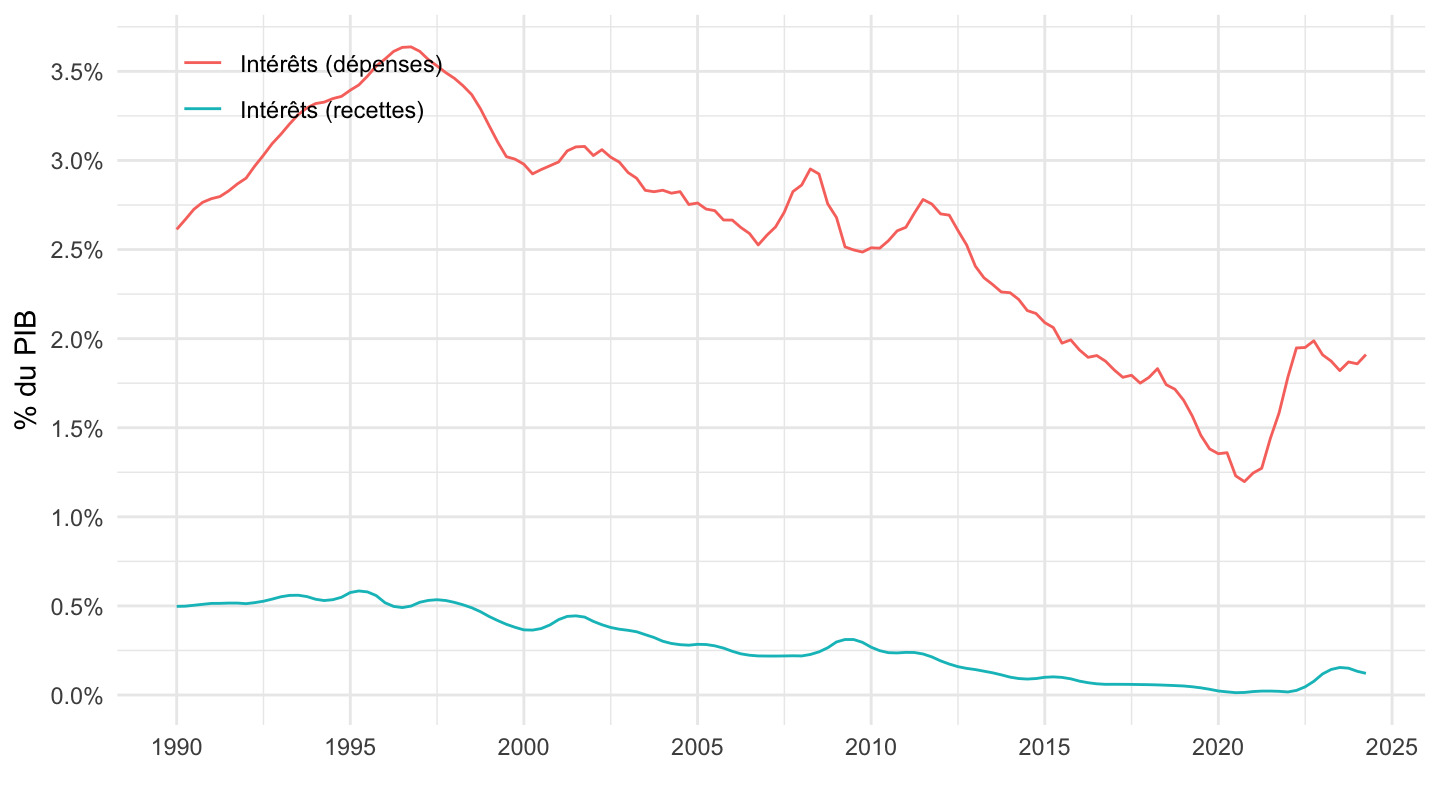
2008-
Code
t_compteapu_val %>%
  filter(column %in% c(21, 9, 33),
         date >= as.Date("2008-01-01")) %>%
  spread(column, value) %>%
  transmute(date,
         `Intérêts (dépenses)` = `9`/`33`,
         `Intérêts (recettes)` = `21`/`33`) %>%
  gather(variable, value, -date) %>%
  filter(!is.na(value)) %>%
  ggplot(.) + theme_minimal() + ylab("% du PIB") + xlab("") +
  geom_line(aes(x = date, y = value, color = variable)) +
  theme(legend.title = element_blank(),
        legend.position = c(0.15, 0.9)) +
  scale_x_date(breaks = seq(1950, 2100, 1) %>% paste0("-01-01") %>% as.Date,
               labels = date_format("%Y")) +
  scale_y_continuous(breaks = 0.01*seq(0, 100, .5),
                     labels = scales::percent_format(accuracy = .1))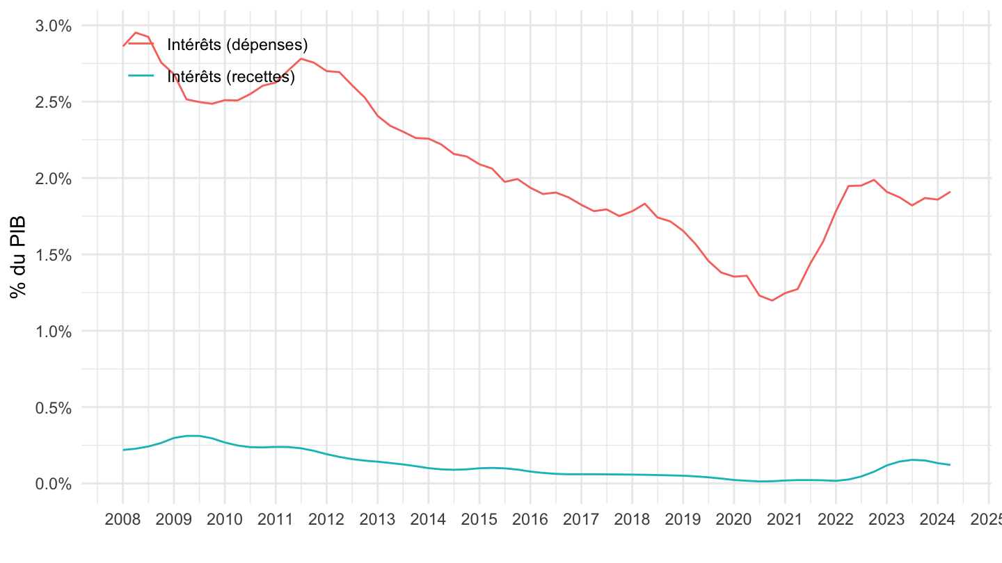
Déficit public (% du PIB)
Déficit total
Code
t_compteapu_val %>%
  filter(column %in% c(34)) %>%
  transmute(date,
         value = value/100) %>%
  gather(variable, value, -date) %>%
  filter(!is.na(value)) %>%
  ggplot(.) + theme_minimal() + ylab("Déficit Public (% du PIB)") + xlab("") +
  geom_line(aes(x = date, y = value)) +
  theme(legend.title = element_blank(),
        legend.position = c(0.15, 0.9)) +
  scale_x_date(breaks = seq(1950, 2100, 5) %>% paste0("-01-01") %>% as.Date,
               labels = date_format("%Y")) +
  scale_y_continuous(breaks = 0.01*seq(-100, 100, 1),
                     labels = scales::percent_format(accuracy = 1))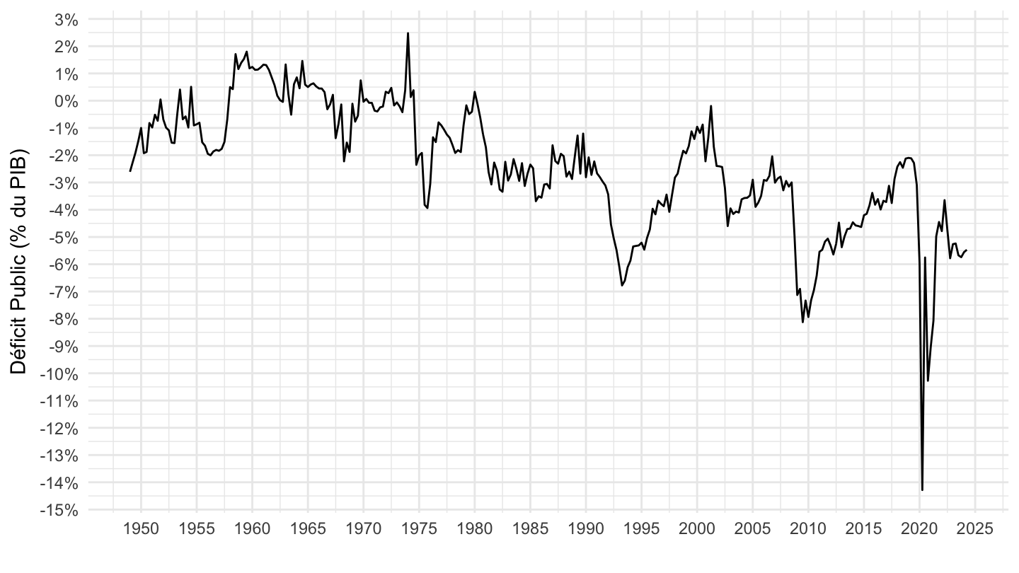
Déficit total, déficit primaire, charges d’intérêt
Tous
Code
t_compteapu_val %>%
  left_join(variable, by = "column") %>%
  select(date, variable, value) %>%
  filter(variable %in% c("D41_d", "D41_r", "PIB", "B9NF")) %>%
  spread(variable, value) %>%
  transmute(date,
            `Déficit total` = B9NF/PIB,
            `Déficit primaire` = (B9NF + D41_d-D41_r)/PIB,
            `Charge d'intérêt` = B9NF/PIB - (B9NF + D41_d-D41_r)/PIB) %>%
  gather(variable, value, -date) %>%
  filter(!is.na(value)) %>%
  ggplot(.) + theme_minimal() + ylab("% du PIB") + xlab("") +
  geom_line(aes(x = date, y = value, color = variable)) +
  theme(legend.title = element_blank(),
        legend.position = c(0.15, 0.2)) +
  scale_x_date(breaks = seq(1950, 2100, 5) %>% paste0("-01-01") %>% as.Date,
               labels = date_format("%Y")) +
  scale_y_continuous(breaks = 0.01*seq(-100, 100, 1),
                     labels = scales::percent_format(accuracy = 1))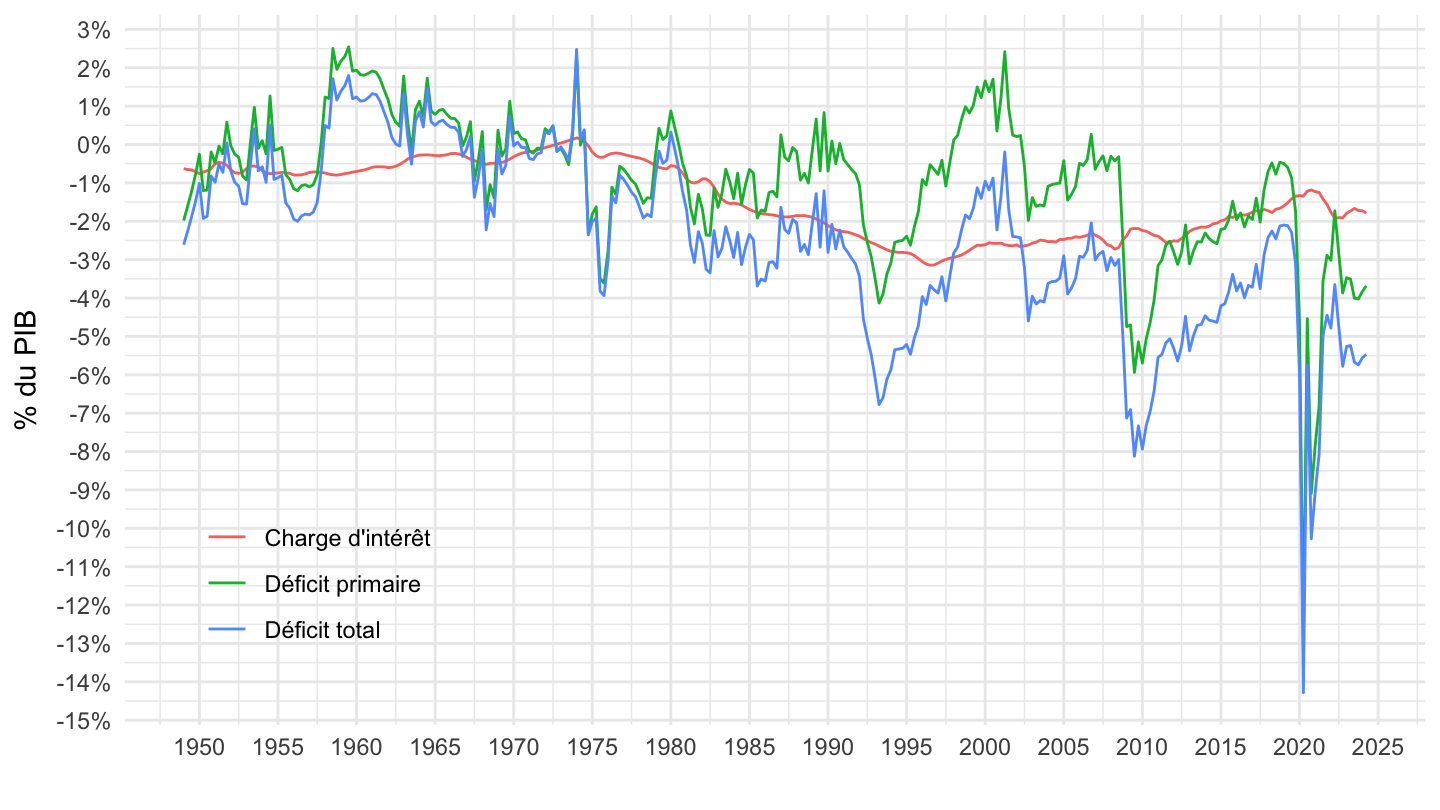
2005-
Code
t_compteapu_val %>%
  left_join(variable, by = "column") %>%
  select(date, variable, value) %>%
  filter(variable %in% c("D41_d", "D41_r", "PIB", "B9NF")) %>%
  filter(date >= as.Date("2005-01-01")) %>%
  spread(variable, value) %>%
  transmute(date,
            `Déficit total` = B9NF/PIB,
            `Déficit primaire` = (B9NF + D41_d-D41_r)/PIB,
            `Charge d'intérêt` = B9NF/PIB - (B9NF + D41_d-D41_r)/PIB) %>%
  gather(variable, value, -date) %>%
  filter(!is.na(value)) %>%
  ggplot(.) + theme_minimal() + ylab("% du PIB") + xlab("") +
  geom_line(aes(x = date, y = value, color = variable)) +
  theme(legend.title = element_blank(),
        legend.position = c(0.15, 0.2)) +
  scale_x_date(breaks = seq(1950, 2100, 2) %>% paste0("-01-01") %>% as.Date,
               labels = date_format("%Y")) +
  scale_y_continuous(breaks = 0.01*seq(-100, 100, 1),
                     labels = scales::percent_format(accuracy = 1))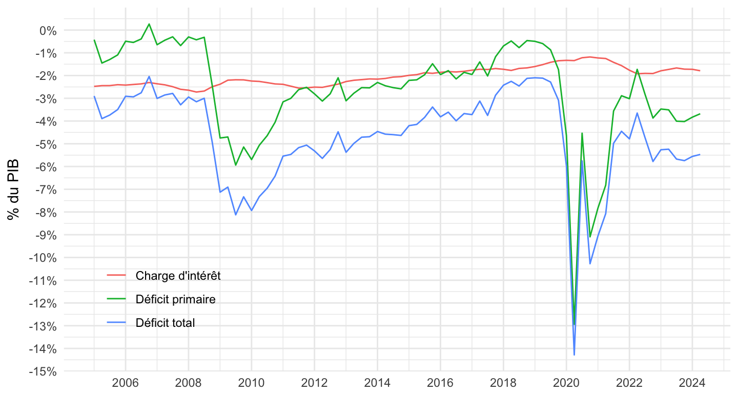
2008-2016
Code
t_compteapu_val %>%
  left_join(variable, by = "column") %>%
  select(date, variable, value) %>%
  filter(variable %in% c("D41_d", "D41_r", "PIB", "B9NF")) %>%
  filter(date >= as.Date("2008-01-01"),
         date <= as.Date("2016-10-01")) %>%
  spread(variable, value) %>%
  transmute(date,
            `Déficit total` = B9NF/PIB,
            `Déficit primaire` = (B9NF + D41_d-D41_r)/PIB,
            `Charge d'intérêt` = B9NF/PIB - (B9NF + D41_d-D41_r)/PIB) %>%
  gather(variable, value, -date) %>%
  filter(!is.na(value)) %>%
  ggplot(.) + theme_minimal() + ylab("% du PIB") + xlab("") +
  geom_line(aes(x = date, y = value, color = variable)) +
  theme(legend.title = element_blank(),
        legend.position = c(0.8, 0.2)) +
  scale_x_date(breaks = seq(1950, 2100, 1) %>% paste0("-01-01") %>% as.Date,
               labels = date_format("%Y")) +
  scale_y_continuous(breaks = 0.01*seq(-100, 100, 1),
                     labels = scales::percent_format(accuracy = 1))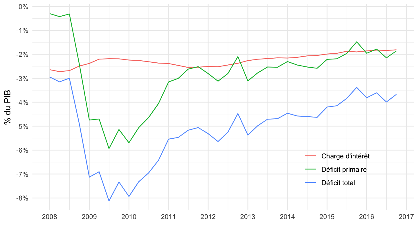
2015-
Code
t_compteapu_val %>%
  left_join(variable, by = "column") %>%
  select(date, variable, value) %>%
  filter(variable %in% c("D41_d", "D41_r", "PIB", "B9NF")) %>%
  filter(date >= as.Date("2015-01-01")) %>%
  spread(variable, value) %>%
  transmute(date,
            `Déficit total` = B9NF/PIB,
            `Déficit primaire` = (B9NF + D41_d-D41_r)/PIB,
            `Charge d'intérêt` = B9NF/PIB - (B9NF + D41_d-D41_r)/PIB) %>%
  gather(variable, value, -date) %>%
  filter(!is.na(value)) %>%
  ggplot(.) + theme_minimal() + ylab("% du PIB") + xlab("") +
  geom_line(aes(x = date, y = value, color = variable)) +
  theme(legend.title = element_blank(),
        legend.position = c(0.8, 0.2)) +
  scale_x_date(breaks = seq(1950, 2100, 1) %>% paste0("-01-01") %>% as.Date,
               labels = date_format("%Y")) +
  scale_y_continuous(breaks = 0.01*seq(-100, 100, 1),
                     labels = scales::percent_format(accuracy = 1))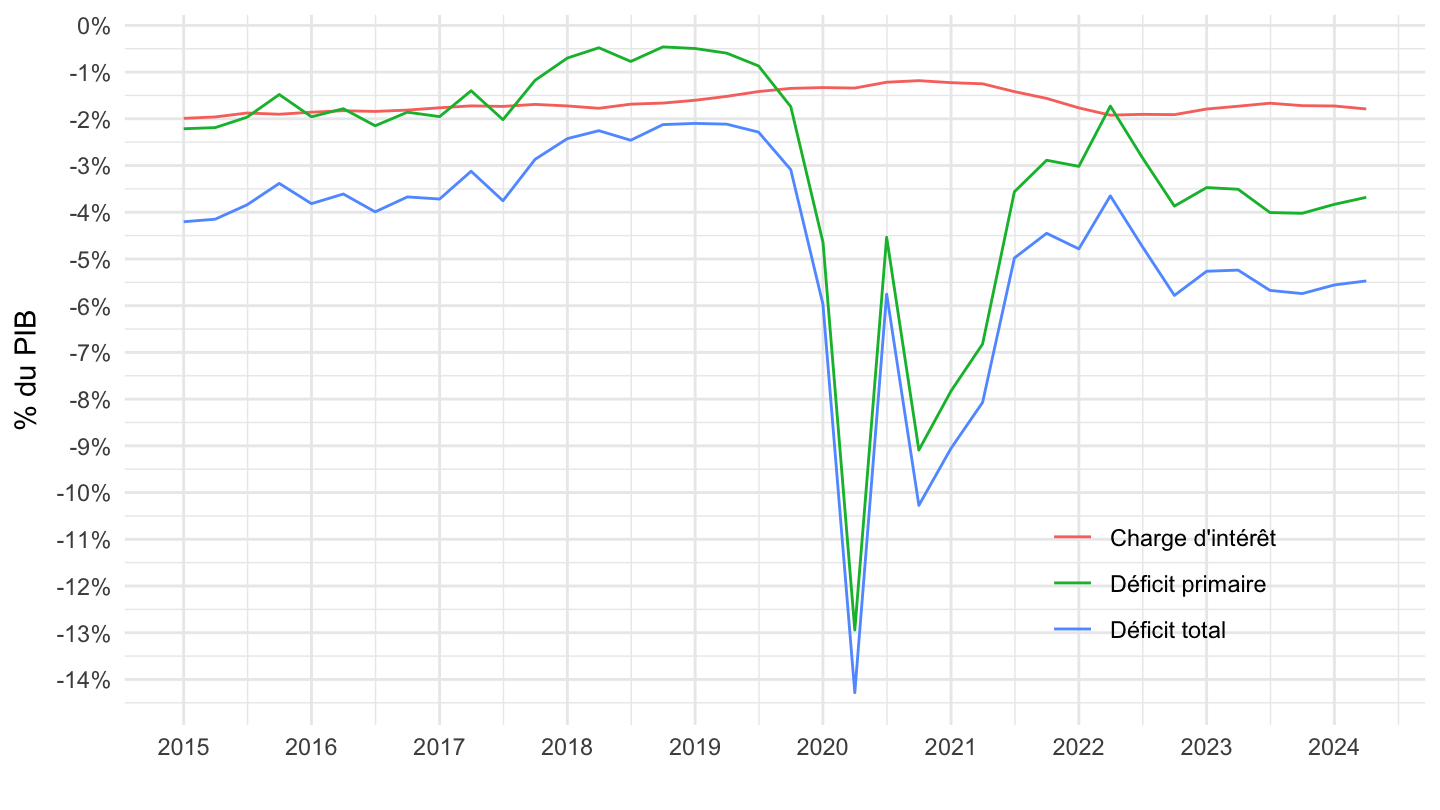
2017T2-
Code
df <- t_compteapu_val %>%
  left_join(variable, by = "column") %>%
  select(date, variable, value) %>%
  filter(variable %in% c("D41_d", "D41_r", "PIB", "B9NF")) %>%
  filter(date >= as.Date("2017-04-01")) %>%
  spread(variable, value) %>%
  transmute(date,
            `Déficit total` = B9NF/PIB,
            `Déficit primaire` = (B9NF + D41_d-D41_r)/PIB,
            `Charge d'intérêt` = B9NF/PIB - (B9NF + D41_d-D41_r)/PIB) %>%
  gather(variable, value, -date) %>%
  filter(!is.na(value)) %>%
  mutate(date = zoo::as.yearqtr(paste0(year(date), " Q", quarter(date))))

ggplot(data = df) + theme_minimal() + ylab("% du PIB") + xlab("") +
  geom_line(aes(x = date, y = value, color = variable)) +
  theme(axis.text.x = element_text(angle = 45, vjust = 1, hjust = 1)) +
  theme(legend.title = element_blank(),
        legend.position = c(0.8, 0.2)) +
  scale_x_yearqtr(labels = date_format("%Y T%q"),
                  breaks = seq(from = min(df$date), to = max(df$date), by = 0.5)) +
  scale_y_continuous(breaks = 0.01*seq(-100, 100, 1),
                     labels = scales::percent_format(accuracy = 1))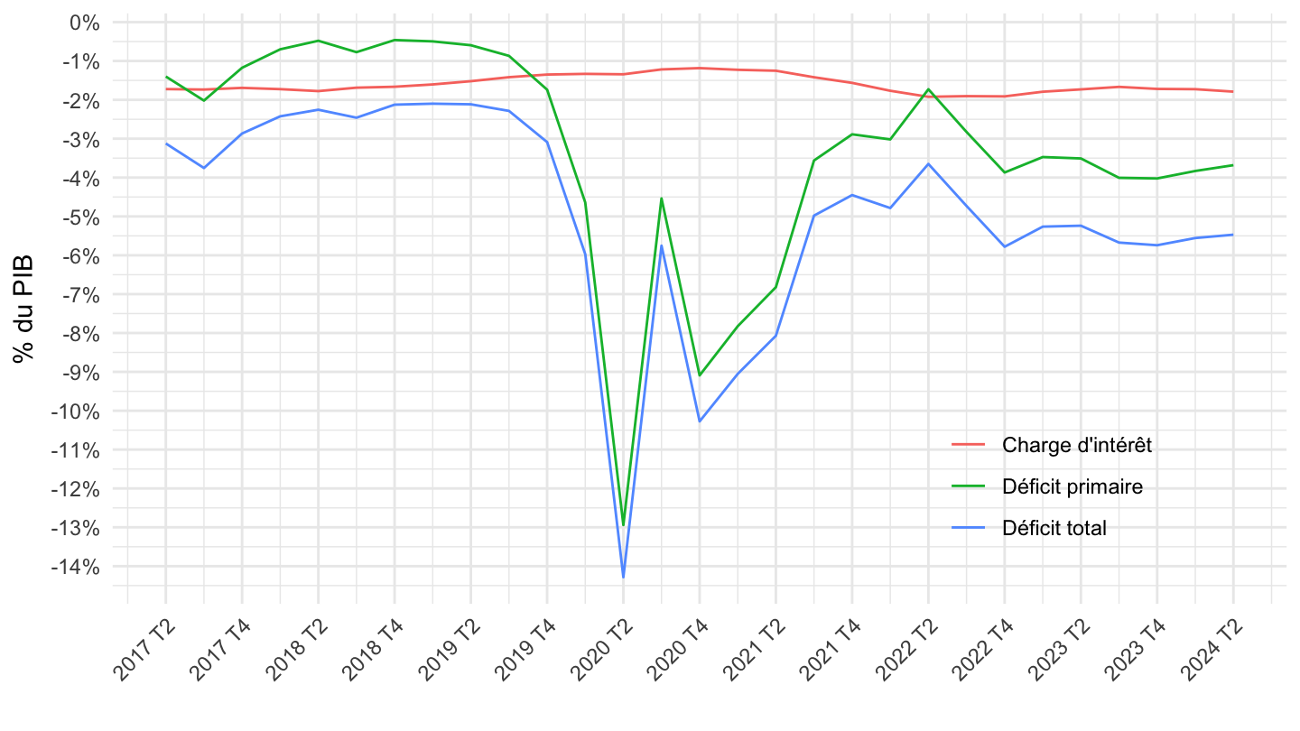
2019-
Code
df <- t_compteapu_val %>%
  left_join(variable, by = "column") %>%
  select(date, variable, value) %>%
  filter(variable %in% c("D41_d", "D41_r", "PIB", "B9NF")) %>%
  filter(date >= as.Date("2019-01-01")) %>%
  spread(variable, value) %>%
  transmute(date,
            `Déficit total` = B9NF/PIB,
            `Déficit primaire` = (B9NF + D41_d-D41_r)/PIB,
            `Charge d'intérêt` = B9NF/PIB - (B9NF + D41_d-D41_r)/PIB) %>%
  gather(variable, value, -date) %>%
  filter(!is.na(value)) %>%
  mutate(date = zoo::as.yearqtr(paste0(year(date), " Q", quarter(date))))

ggplot(data = df) + theme_minimal() + ylab("% du PIB") + xlab("") +
  geom_line(aes(x = date, y = value, color = variable)) +
  theme(axis.text.x = element_text(angle = 45, vjust = 1, hjust = 1)) +
  theme(legend.title = element_blank(),
        legend.position = c(0.8, 0.2)) +
  scale_x_yearqtr(labels = date_format("%Y T%q"),
                  breaks = seq(from = min(df$date), to = max(df$date), by = 0.25)) +
  scale_y_continuous(breaks = 0.01*seq(-100, 100, 1),
                     labels = scales::percent_format(accuracy = 1))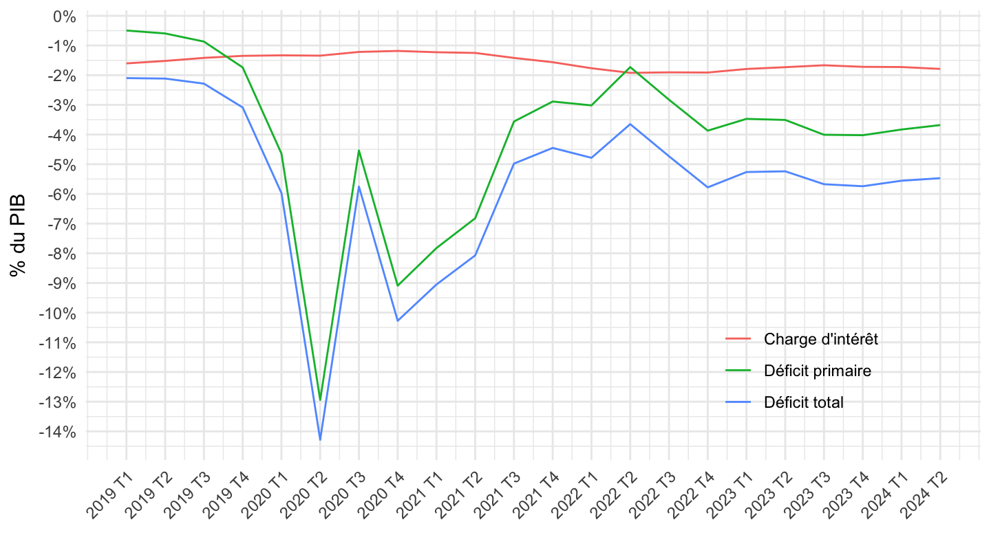
Déficit total, déficit primaire
Tous
Code
df <- t_compteapu_val %>%
  left_join(variable, by = "column") %>%
  select(date, variable, value) %>%
  filter(variable %in% c("D41_d", "D41_r", "PIB", "B9NF")) %>%
  spread(variable, value) %>%
  transmute(date,
            `Déficit total` = B9NF/PIB,
            `Déficit primaire` = (B9NF + D41_d-D41_r)/PIB) %>%
  gather(variable, value, -date) %>%
  filter(!is.na(value)) %>%
  mutate(date = zoo::as.yearqtr(paste0(year(date), " Q", quarter(date))))

ggplot(data = df) + theme_minimal() + ylab("% du PIB") + xlab("") +
  geom_line(aes(x = date, y = value, color = variable)) +
  theme(legend.title = element_blank(),
        legend.position = c(0.15, 0.2)) +
  scale_x_yearqtr(labels = date_format("%Y Q%q")) +
  scale_y_continuous(breaks = 0.01*seq(-100, 100, 1),
                     labels = scales::percent_format(accuracy = 1))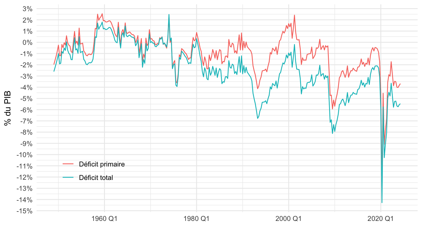
2005-
Code
t_compteapu_val %>%
  left_join(variable, by = "column") %>%
  select(date, variable, value) %>%
  filter(variable %in% c("D41_d", "D41_r", "PIB", "B9NF")) %>%
  filter(date >= as.Date("2005-01-01")) %>%
  spread(variable, value) %>%
  transmute(date,
            `Déficit total` = B9NF/PIB,
            `Déficit primaire` = (B9NF + D41_d-D41_r)/PIB) %>%
  gather(variable, value, -date) %>%
  filter(!is.na(value)) %>%
  ggplot(.) + theme_minimal() + ylab("% du PIB") + xlab("") +
  geom_line(aes(x = date, y = value, color = variable)) +
  theme(legend.title = element_blank(),
        legend.position = c(0.15, 0.2)) +
  scale_x_date(breaks = seq(1950, 2100, 2) %>% paste0("-01-01") %>% as.Date,
               labels = date_format("%Y")) +
  scale_y_continuous(breaks = 0.01*seq(-100, 100, 1),
                     labels = scales::percent_format(accuracy = 1))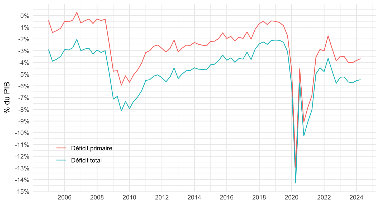
2008-2016
Code
t_compteapu_val %>%
  left_join(variable, by = "column") %>%
  select(date, variable, value) %>%
  filter(variable %in% c("D41_d", "D41_r", "PIB", "B9NF")) %>%
  filter(date >= as.Date("2008-01-01"),
         date <= as.Date("2016-10-01")) %>%
  spread(variable, value) %>%
  transmute(date,
            `Déficit total` = B9NF/PIB,
            `Déficit primaire` = (B9NF + D41_d-D41_r)/PIB) %>%
  gather(variable, value, -date) %>%
  filter(!is.na(value)) %>%
  ggplot(.) + theme_minimal() + ylab("% du PIB") + xlab("") +
  geom_line(aes(x = date, y = value, color = variable)) +
  theme(legend.title = element_blank(),
        legend.position = c(0.8, 0.2)) +
  scale_x_date(breaks = seq(1950, 2100, 1) %>% paste0("-01-01") %>% as.Date,
               labels = date_format("%Y")) +
  scale_y_continuous(breaks = 0.01*seq(-100, 100, 1),
                     labels = scales::percent_format(accuracy = 1))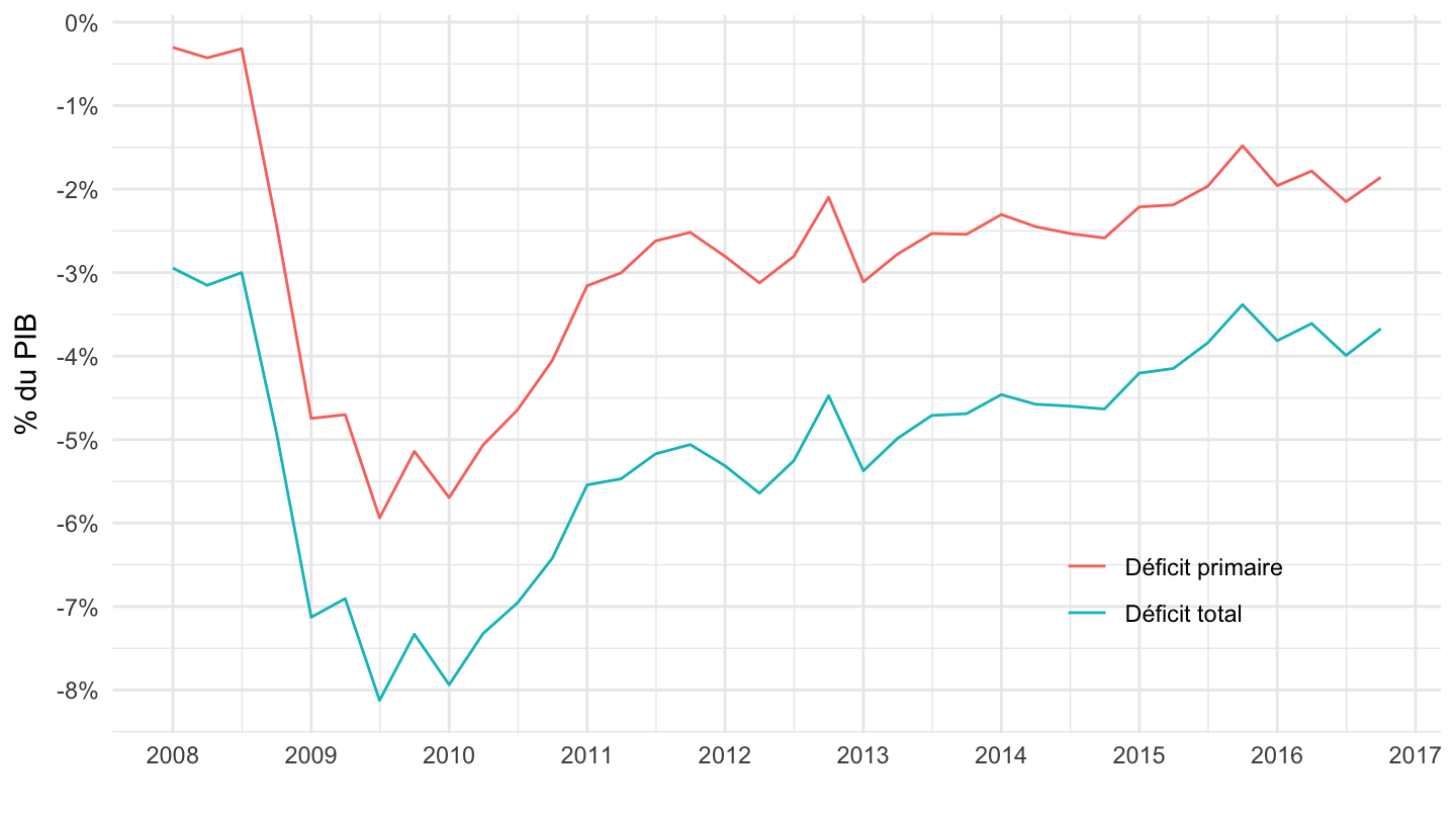
2015-
Code
t_compteapu_val %>%
  left_join(variable, by = "column") %>%
  select(date, variable, value) %>%
  filter(variable %in% c("D41_d", "D41_r", "PIB", "B9NF")) %>%
  filter(date >= as.Date("2015-01-01")) %>%
  spread(variable, value) %>%
  transmute(date,
            `Déficit total` = B9NF/PIB,
            `Déficit primaire` = (B9NF + D41_d-D41_r)/PIB) %>%
  gather(variable, value, -date) %>%
  filter(!is.na(value)) %>%
  ggplot(.) + theme_minimal() + ylab("% du PIB") + xlab("") +
  geom_line(aes(x = date, y = value, color = variable)) +
  theme(legend.title = element_blank(),
        legend.position = c(0.8, 0.2)) +
  scale_x_date(breaks = seq(1950, 2100, 1) %>% paste0("-01-01") %>% as.Date,
               labels = date_format("%Y")) +
  scale_y_continuous(breaks = 0.01*seq(-100, 100, 1),
                     labels = scales::percent_format(accuracy = 1))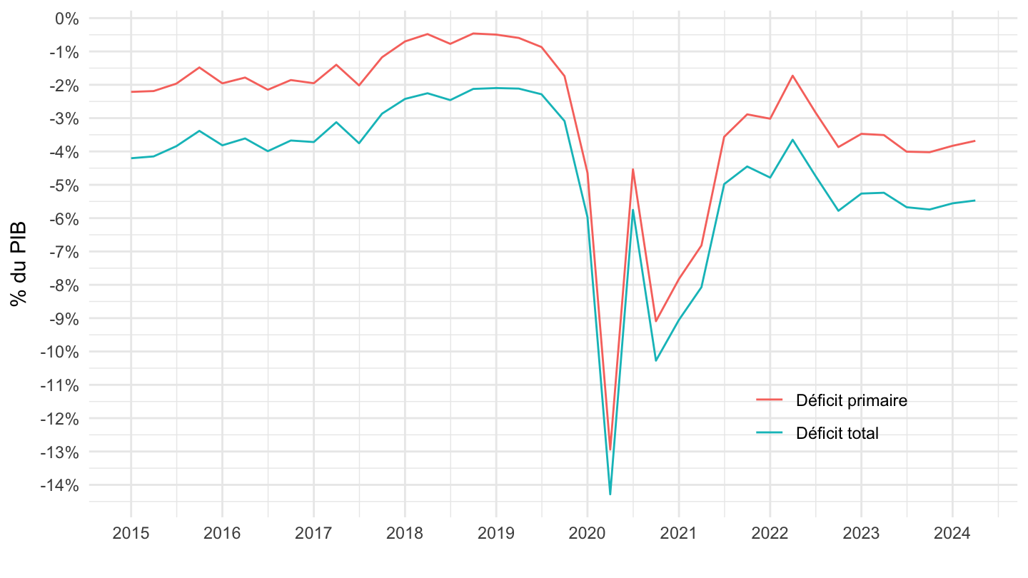
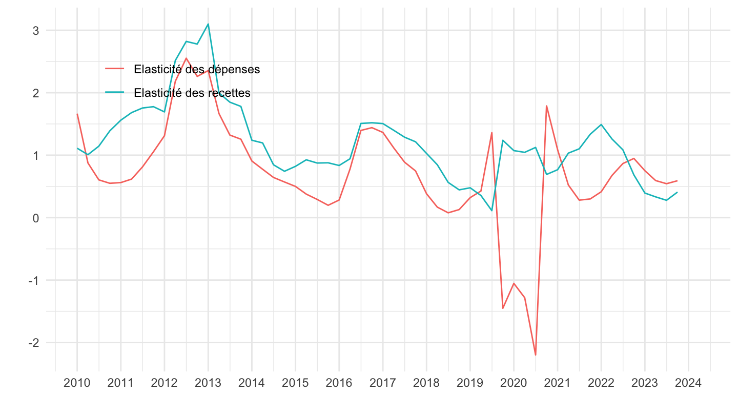
Elasticité des recettes au PIB
1980-
Code
t_compteapu_val %>%
  left_join(variable, by = "column") %>%
  filter(operation %in% c("PIB", "DEPENSES", "RECETTES")) %>%
  select(operation, date, value) %>%
  arrange(date) %>%
  spread(operation, value) %>%
  na.omit %>%
  mutate(DEPENSES_roll = rollsum(DEPENSES, k = 4, fill = NA),
         RECETTES_roll = rollsum(RECETTES, k = 4, fill = NA),
         PIB_roll = rollsum(PIB, k = 4, fill = NA)) %>%
  mutate(croissance_PIB = PIB_roll/lag(PIB_roll, 4)-1,
         croissance_RECETTES = RECETTES_roll/lag(RECETTES_roll, 4)-1,
         croissance_DEPENSES = DEPENSES_roll/lag(DEPENSES_roll, 4)-1,
         `Elasticité des recettes` = croissance_RECETTES/croissance_PIB,
         `Elasticité des dépenses` = croissance_DEPENSES/croissance_PIB) %>%
  select(date, `Elasticité des recettes`, `Elasticité des dépenses`) %>%
  gather(variable, value, -date) %>%
  ggplot(.) + theme_minimal() + ylab("") + xlab("") +
  geom_line(aes(x = date, y = value, color = variable)) +
  theme(legend.title = element_blank(),
        legend.position = c(0.2, 0.8)) +
  scale_x_date(breaks = seq(1950, 2100, 5) %>% paste0("-01-01") %>% as.Date,
               labels = date_format("%Y"))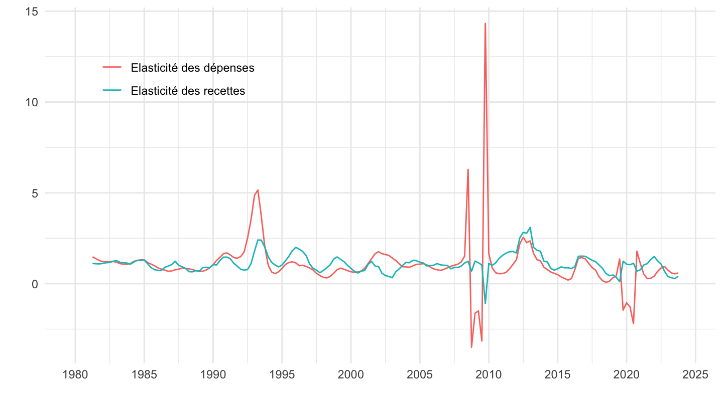
2010-
Code
t_compteapu_val %>%
  left_join(variable, by = "column") %>%
  filter(operation %in% c("PIB", "DEPENSES", "RECETTES")) %>%
  select(operation, date, value) %>%
  arrange(date) %>%
  spread(operation, value) %>%
  na.omit %>%
  mutate(DEPENSES_roll = rollsum(DEPENSES, k = 4, fill = NA),
         RECETTES_roll = rollsum(RECETTES, k = 4, fill = NA),
         PIB_roll = rollsum(PIB, k = 4, fill = NA)) %>%
  mutate(croissance_PIB = PIB_roll/lag(PIB_roll, 4)-1,
         croissance_RECETTES = RECETTES_roll/lag(RECETTES_roll, 4)-1,
         croissance_DEPENSES = DEPENSES_roll/lag(DEPENSES_roll, 4)-1,
         `Elasticité des recettes` = croissance_RECETTES/croissance_PIB,
         `Elasticité des dépenses` = croissance_DEPENSES/croissance_PIB) %>%
  select(date, `Elasticité des recettes`, `Elasticité des dépenses`) %>%
  gather(variable, value, -date) %>%
  filter(date >= as.Date("2010-01-01")) %>%
  ggplot(.) + theme_minimal() + ylab("") + xlab("") +
  geom_line(aes(x = date, y = value, color = variable)) +
  theme(legend.title = element_blank(),
        legend.position = c(0.2, 0.8)) +
  scale_x_date(breaks = seq(1950, 2100, 1) %>% paste0("-01-01") %>% as.Date,
               labels = date_format("%Y"))