Key indicators and growth rates of selected transactions
Data - Eurostat
Info
Last observation: Quarterly: 2026Q1 (N = 88)
First observation: Quarterly: 1980Q1 (N = 9)
Last data update: 23 jul 2026, 22:44. Last compile: 24 jul 2026, 03:07
Structure
na_item
Code
load_data("eurostat/na_item.RData")
nasq_10_ki %>%

  group_by(na_item, Na_item) %>%
  summarise(Nobs = n()) %>%
  arrange(-Nobs) %>%
print_table_conditional()| na_item | Na_item | Nobs |
|---|---|---|
| B2G_B3G_RAT_S11 | Gross profit share of non-financial corporations (B2G_B3G/B1G*100) | 4912 |
| IRG_S11 | Gross investment rate of non-financial corporations (P51G/B1G*100) | 4828 |
| SRG_S14_S15 | Gross household saving rate (B8G/(B6G+D8Net)*100) | 4588 |
| IRG_S14_S15 | Gross investment rate of households (P51G/(B6G+D8Net)*100) | 4511 |
| B6G_R_HAB_2010 | Gross disposable income of households in real terms per capita (2010=100) | 2075 |
| B6G_R_HAB_GR | Gross disposable income of households in real terms per capita (percentage change on previous period) | 2025 |
| NFW_S14_S15 | Household net financial assets ratio (BF90/(B6G+D8net)*100) | 1949 |
| B7G_R_HAB_2010 | Adjusted gross disposable income of households in real terms per capita (2010=100) | 324 |
| B7G_R_HAB_GR | Adjusted gross disposable income of households in real terms per capita (percentage change on previous period) | 321 |
| P4_R_HAB_2010 | Actual final consumption in real terms per capita (2010=100) | 108 |
| B7G_N_HAB_GR | Adjusted gross disposable income of households in nominal terms per capita (percentage change on previous period) | 107 |
| P4_R_HAB_GR | Actual final consumption in real terms per capita (percentage change on previous period) | 107 |
Adjusted gross disposable income of households in real terms per capita (2010=100) - B7G
France, Germany, Spain, Italy, Europe
All
Code
nasq_10_ki %>%
  filter(geo %in% c("FR", "DE", "IT", "ES", "EA20"),
         na_item == "B7G_R_HAB_2010",
         s_adj == "SCA") %>%
  quarter_to_date %>%

  mutate(Geo = ifelse(geo == "EA20", "Europe", Geo)) %>%
  left_join(colors, by = c("Geo" = "country")) %>%
  ggplot + theme_minimal() + xlab("") + ylab("") +
  geom_line(aes(x = date, y = values, color = color)) +
  scale_color_identity() + add_2flags +
  scale_x_date(breaks = as.Date(paste0(seq(1940, 2100, 2), "-01-01")),
               labels = date_format("%Y")) +
  scale_y_log10(breaks = seq(0, 1000, 5))
1999-
Code
nasq_10_ki %>%
  filter(geo %in% c("FR", "DE", "IT", "ES", "EA20"),
         na_item == "B7G_R_HAB_2010",
         s_adj == "SCA") %>%
  quarter_to_date %>%
  filter(date >= as.Date("1999-01-01")) %>%

  group_by(geo) %>%
  arrange(date) %>%
  mutate(values = 100*values/values[1]) %>%
  mutate(Geo = ifelse(geo == "EA20", "Europe", Geo)) %>%
  left_join(colors, by = c("Geo" = "country")) %>%
  ggplot + theme_minimal() + xlab("") + ylab("") +
  geom_line(aes(x = date, y = values, color = color)) +
  scale_color_identity() + add_2flags +
  scale_x_date(breaks = as.Date(paste0(seq(1999, 2100, 2), "-01-01")),
               labels = date_format("%Y")) +
  scale_y_log10(breaks = seq(0, 1000, 5))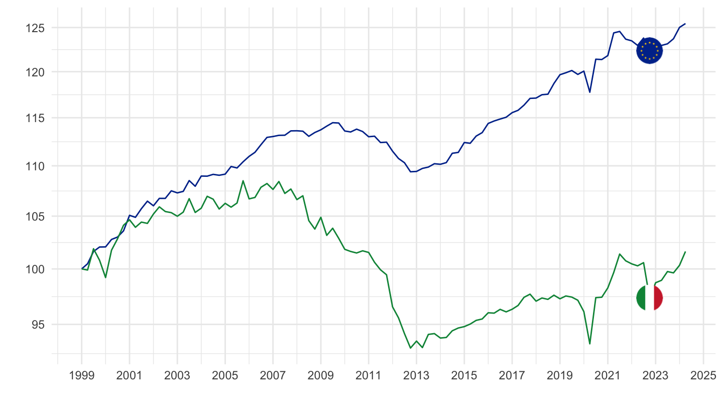
2010-
Code
nasq_10_ki %>%
  filter(geo %in% c("FR", "DE", "IT", "ES", "EA20"),
         na_item == "B7G_R_HAB_2010",
         s_adj == "SCA") %>%
  quarter_to_date %>%
  filter(date >= as.Date("2010-01-01")) %>%

  mutate(Geo = ifelse(geo == "EA20", "Europe", Geo)) %>%
  left_join(colors, by = c("Geo" = "country")) %>%
  ggplot + theme_minimal() + xlab("") + ylab("") +
  geom_line(aes(x = date, y = values, color = color)) +
  scale_color_identity() + add_2flags +
  scale_x_date(breaks = as.Date(paste0(seq(1940, 2100, 2), "-01-01")),
               labels = date_format("%Y")) +
  scale_y_log10(breaks = seq(0, 1000, 5))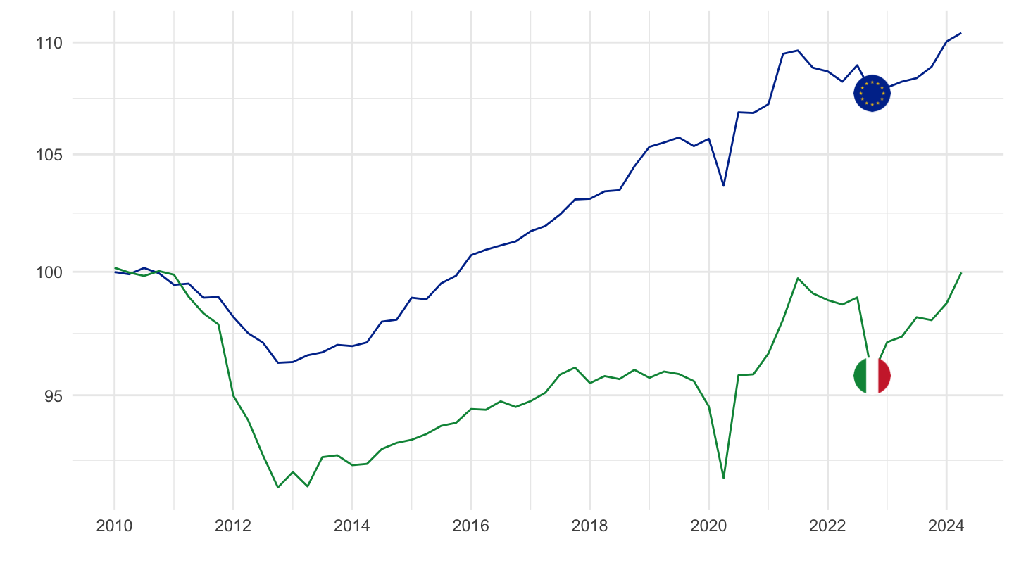
Gross disposable income of households in real terms per capita (2010=100) - B6G
France, Germany, Spain, Italy, Europe
All
Code
nasq_10_ki %>%
  filter(geo %in% c("FR", "DE", "IT", "ES", "EA20"),
         na_item == "B6G_R_HAB_2010",
         s_adj == "SCA") %>%
  quarter_to_date %>%

  mutate(Geo = ifelse(geo == "EA20", "Europe", Geo)) %>%
  left_join(colors, by = c("Geo" = "country")) %>%
  ggplot + theme_minimal() + xlab("") + ylab("") +
  geom_line(aes(x = date, y = values, color = color)) +
  scale_color_identity() + add_5flags +
  scale_x_date(breaks = as.Date(paste0(seq(1940, 2100, 5), "-01-01")),
               labels = date_format("%Y")) +
  scale_y_log10(breaks = seq(0, 1000, 5))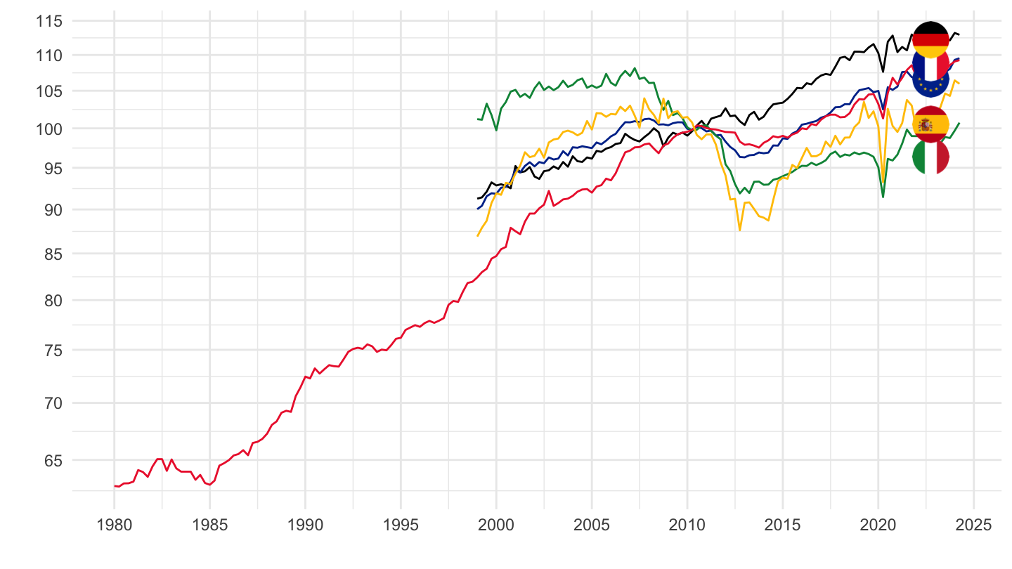
1999-
Code
nasq_10_ki %>%
  filter(geo %in% c("FR", "DE", "IT", "ES", "EA20"),
         na_item == "B6G_R_HAB_2010",
         s_adj == "SCA") %>%
  quarter_to_date %>%
  filter(date >= as.Date("1999-01-01")) %>%

  group_by(geo) %>%
  arrange(date) %>%
  mutate(values = 100*values/values[1]) %>%
  mutate(Geo = ifelse(geo == "EA20", "Europe", Geo)) %>%
  left_join(colors, by = c("Geo" = "country")) %>%
  ggplot + theme_minimal() + xlab("") + ylab("") +
  geom_line(aes(x = date, y = values, color = color)) +
  scale_color_identity() + add_5flags +
  scale_x_date(breaks = as.Date(paste0(seq(1999, 2100, 5), "-01-01")),
               labels = date_format("%Y")) +
  scale_y_log10(breaks = seq(0, 1000, 5))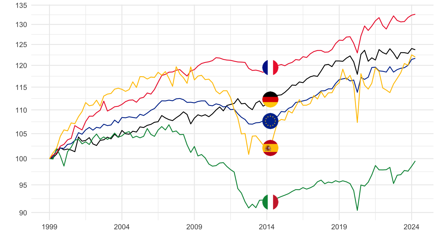
2010-
Code
nasq_10_ki %>%
  filter(geo %in% c("FR", "DE", "IT", "ES", "EA20"),
         na_item == "B6G_R_HAB_2010",
         s_adj == "SCA") %>%
  quarter_to_date %>%
  filter(date >= as.Date("2010-01-01")) %>%

  mutate(Geo = ifelse(geo == "EA20", "Europe", Geo)) %>%
  left_join(colors, by = c("Geo" = "country")) %>%
  ggplot + theme_minimal() + xlab("") + ylab("") +
  geom_line(aes(x = date, y = values, color = color)) +
  scale_color_identity() + add_5flags +
  scale_x_date(breaks = as.Date(paste0(seq(1940, 2100, 2), "-01-01")),
               labels = date_format("%Y")) +
  scale_y_log10(breaks = seq(0, 1000, 5))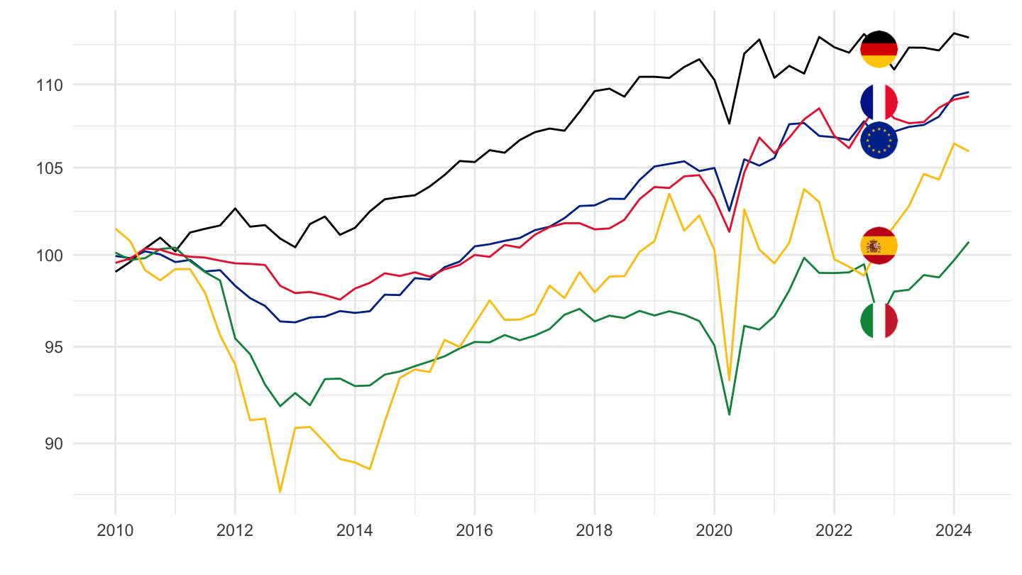
Gross profit share of non-financial corporations (B2G_B3G/B1Q*100)
France, Germany, Spain, Italy, Europe
All
Code
nasq_10_ki %>%
  filter(geo %in% c("FR", "DE", "IT", "ES", "EA20"),
         na_item == "B2G_B3G_RAT_S11",
         s_adj == "SCA") %>%
  quarter_to_date %>%
  mutate(values = values/100) %>%

  mutate(Geo = ifelse(geo == "EA20", "Europe", Geo)) %>%
  left_join(colors, by = c("Geo" = "country")) %>%
  ggplot + theme_minimal() + xlab("") + ylab("") +
  geom_line(aes(x = date, y = values, color = color)) +
  scale_color_identity() + add_5flags +
  scale_x_date(breaks = as.Date(paste0(seq(1940, 2100, 5), "-01-01")),
               labels = date_format("%Y")) +
  scale_y_continuous(breaks = 0.01*seq(0, 100, 5),
                labels = percent_format(a = 1))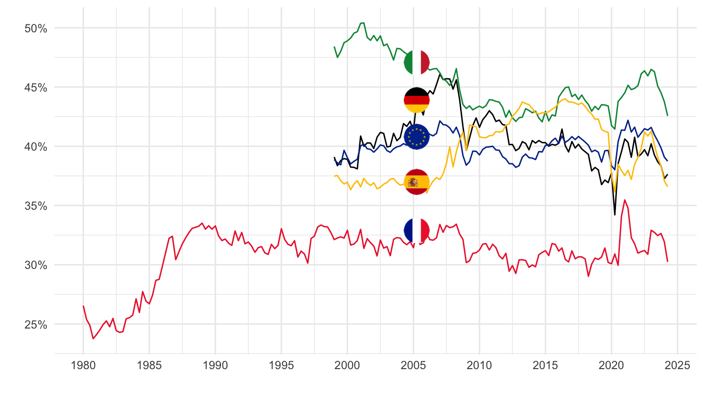
1999-
Code
nasq_10_ki %>%
  filter(geo %in% c("FR", "DE", "IT", "ES", "EA20"),
         na_item == "B2G_B3G_RAT_S11",
         s_adj == "SCA") %>%
  quarter_to_date %>%
  mutate(values = values/100) %>%

  mutate(Geo = ifelse(geo == "EA20", "Europe", Geo)) %>%
  left_join(colors, by = c("Geo" = "country")) %>%
  filter(date >= as.Date("1999-01-01")) %>%
  ggplot + theme_minimal() + xlab("") + ylab("") +
  geom_line(aes(x = date, y = values, color = color)) +
  scale_color_identity() + add_5flags +
  scale_x_date(breaks = as.Date(paste0(seq(1940, 2100, 2), "-01-01")),
               labels = date_format("%Y")) +
  scale_y_continuous(breaks = 0.01*seq(0, 100, 2),
                labels = percent_format(a = 1))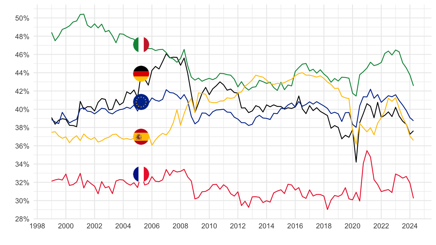
2015-
Code
nasq_10_ki %>%
  filter(geo %in% c("FR", "DE", "IT", "ES", "EA20"),
         na_item == "B2G_B3G_RAT_S11",
         s_adj == "SCA") %>%
  quarter_to_date %>%
  mutate(values = values/100) %>%

  mutate(Geo = ifelse(geo == "EA20", "Europe", Geo)) %>%
  left_join(colors, by = c("Geo" = "country")) %>%
  filter(date >= as.Date("2015-01-01")) %>%
  ggplot + theme_minimal() + xlab("") + ylab("") +
  geom_line(aes(x = date, y = values, color = color)) +
  scale_color_identity() + add_5flags +
  scale_x_date(breaks = as.Date(paste0(seq(1940, 2100, 1), "-01-01")),
               labels = date_format("%Y")) +
  scale_y_continuous(breaks = 0.01*seq(0, 100, 1),
                labels = percent_format(a = 1))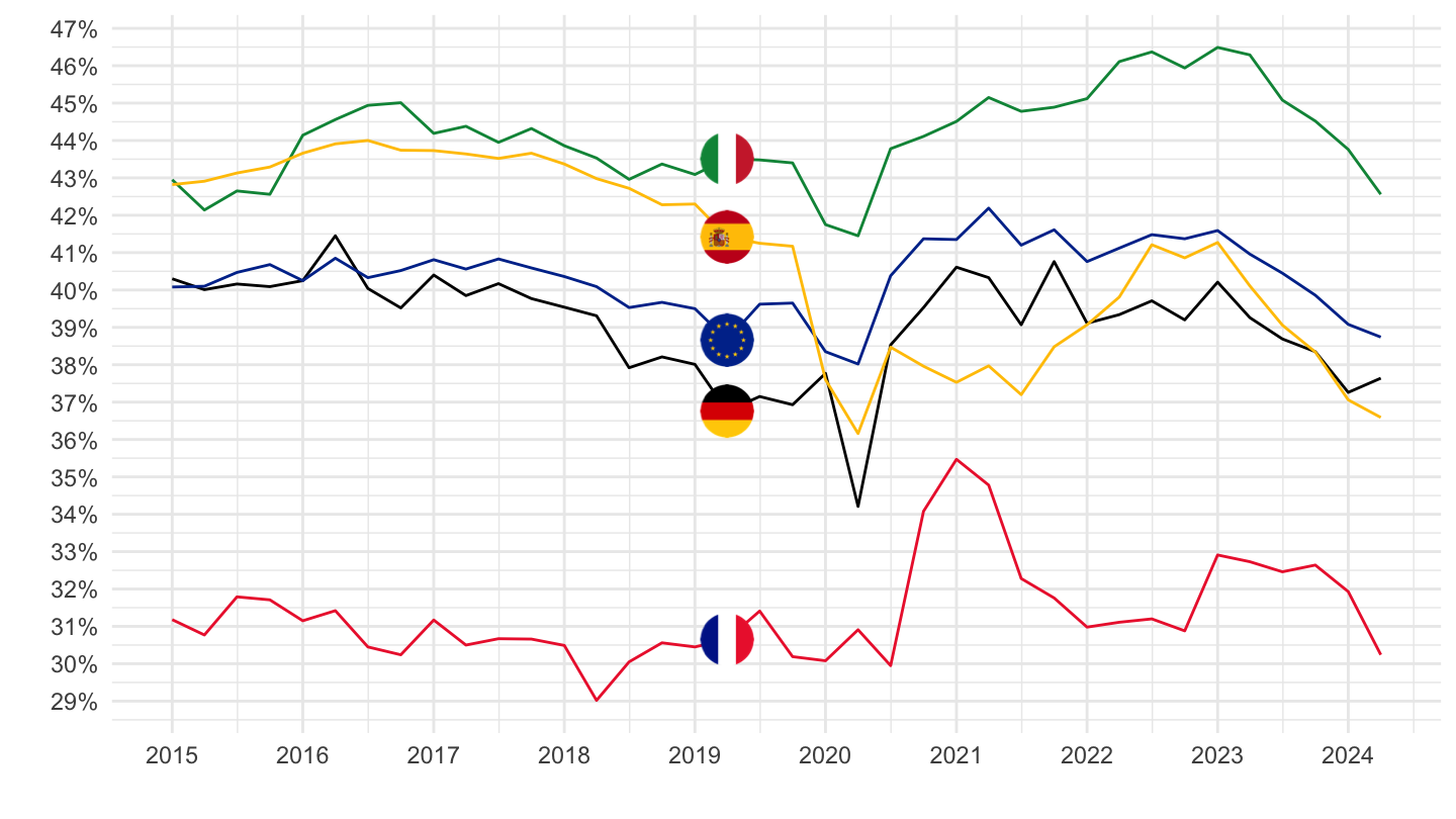
Gross household saving rate (B8G/(B6G+D8Net)*100)
France, Germany, Spain, Italy, Europe
All
Code
nasq_10_ki %>%
  filter(geo %in% c("FR", "DE", "IT", "ES", "EA20"),
         na_item == "SRG_S14_S15",
         s_adj == "SCA") %>%
  quarter_to_date %>%
  mutate(values = values/100) %>%

  mutate(Geo = ifelse(geo == "EA20", "Europe", Geo)) %>%
  left_join(colors, by = c("Geo" = "country")) %>%
  ggplot + theme_minimal() + xlab("") + ylab("") +
  geom_line(aes(x = date, y = values, color = color)) +
  scale_color_identity() + add_5flags +
  scale_x_date(breaks = as.Date(paste0(seq(1940, 2100, 5), "-01-01")),
               labels = date_format("%Y")) +
  scale_y_continuous(breaks = 0.01*seq(0, 100, 5),
                labels = percent_format(a = 1))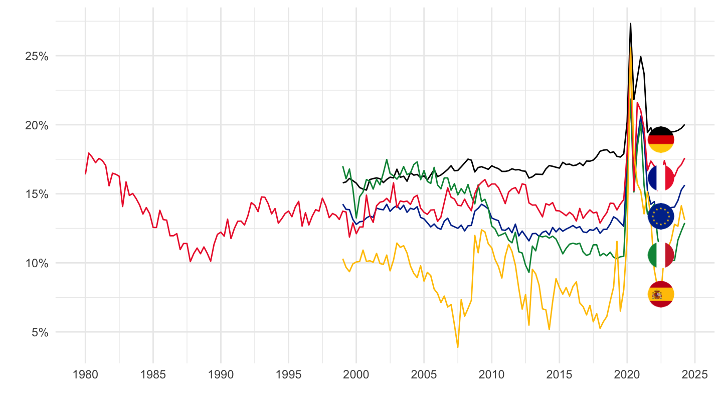
1999-
Code
nasq_10_ki %>%
  filter(geo %in% c("FR", "DE", "IT", "ES", "EA20"),
         na_item == "SRG_S14_S15",
         s_adj == "SCA") %>%
  quarter_to_date %>%
  mutate(values = values/100) %>%

  mutate(Geo = ifelse(geo == "EA20", "Europe", Geo)) %>%
  left_join(colors, by = c("Geo" = "country")) %>%
  filter(date >= as.Date("1999-01-01")) %>%
  ggplot + theme_minimal() + xlab("") + ylab("") +
  geom_line(aes(x = date, y = values, color = color)) +
  scale_color_identity() + add_5flags +
  scale_x_date(breaks = as.Date(paste0(seq(1940, 2100, 2), "-01-01")),
               labels = date_format("%Y")) +
  scale_y_continuous(breaks = 0.01*seq(0, 100, 2),
                labels = percent_format(a = 1))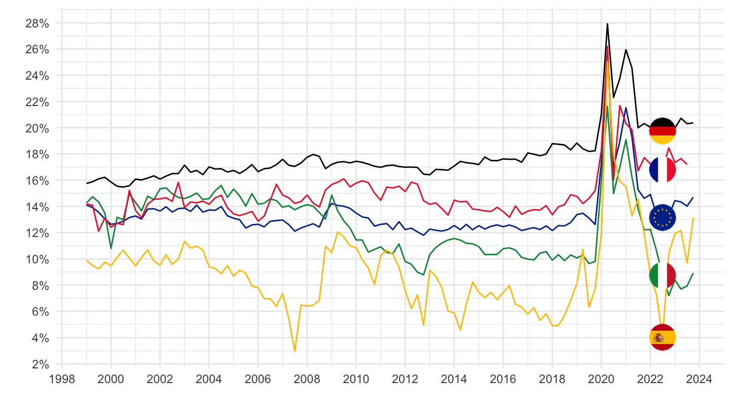
2015-
Code
nasq_10_ki %>%
  filter(geo %in% c("FR", "DE", "IT", "ES", "EA20"),
         na_item == "SRG_S14_S15",
         s_adj == "SCA") %>%
  quarter_to_date %>%
  mutate(values = values/100) %>%

  mutate(Geo = ifelse(geo == "EA20", "Europe", Geo)) %>%
  left_join(colors, by = c("Geo" = "country")) %>%
  filter(date >= as.Date("2015-01-01")) %>%
  ggplot + theme_minimal() + xlab("") + ylab("") +
  geom_line(aes(x = date, y = values, color = color)) +
  scale_color_identity() + add_5flags +
  scale_x_date(breaks = as.Date(paste0(seq(1940, 2100, 1), "-01-01")),
               labels = date_format("%Y")) +
  scale_y_continuous(breaks = 0.01*seq(0, 100, 1),
                labels = percent_format(a = 1))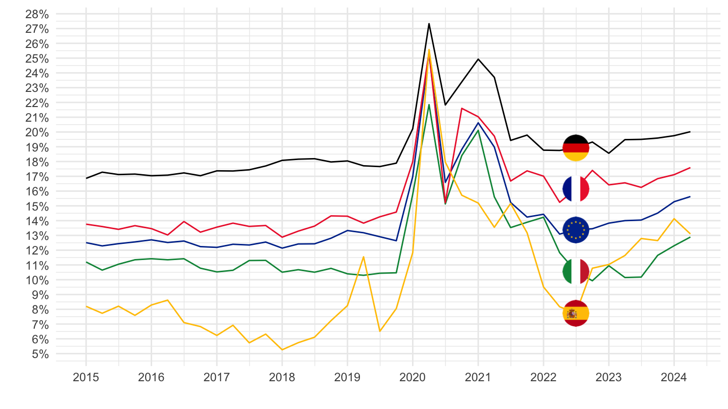
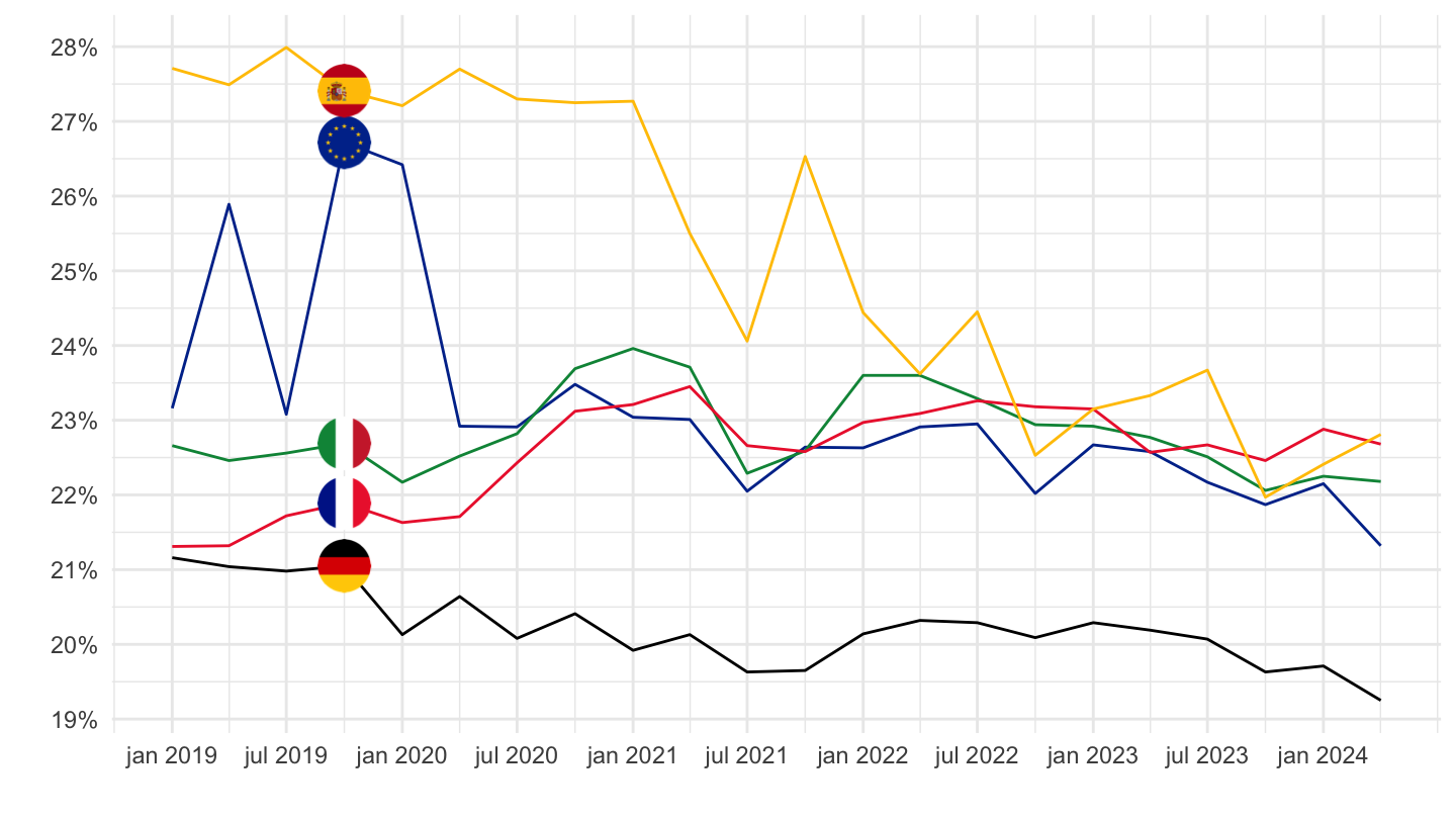
2019-
Code
nasq_10_ki %>%
  filter(geo %in% c("FR", "DE", "IT", "ES", "EA20"),
         na_item == "SRG_S14_S15",
         s_adj == "SCA") %>%
  quarter_to_date %>%
  mutate(values = values/100) %>%

  mutate(Geo = ifelse(geo == "EA20", "Europe", Geo)) %>%
  left_join(colors, by = c("Geo" = "country")) %>%
  filter(date >= as.Date("2019-01-01")) %>%
  ggplot + theme_minimal() + xlab("") + ylab("") +
  geom_line(aes(x = date, y = values, color = color)) +
  scale_color_identity() + add_5flags +
  scale_x_date(breaks = seq.Date(from = as.Date("2018-01-01"), to = as.Date("2100-01-01"), by = "6 months"),
               labels = date_format("%b %Y")) +
  scale_y_continuous(breaks = 0.01*seq(0, 100, 1),
                labels = percent_format(a = 1))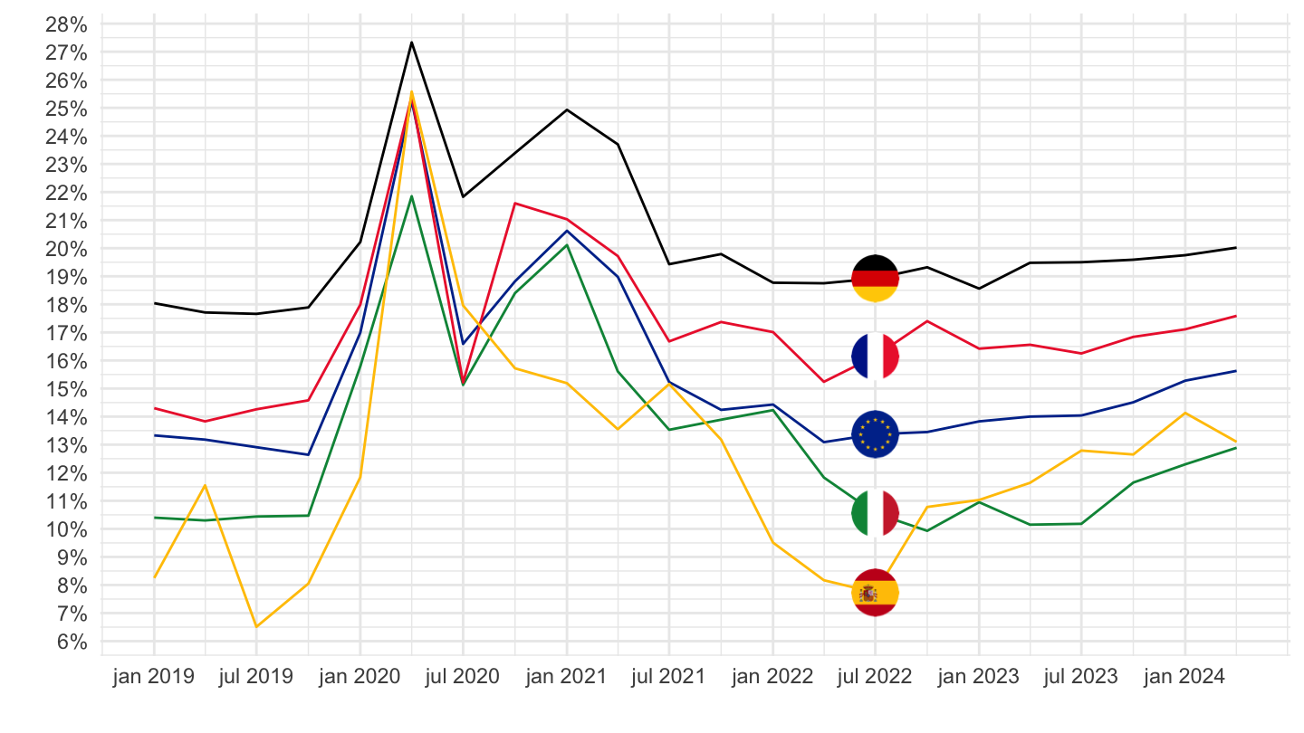
Gross investment rate of households (P51/(B6G+D8Net)*100)
France, Germany, Spain, Italy, Europe
All
Code
nasq_10_ki %>%
  filter(geo %in% c("FR", "DE", "IT", "ES", "EA20"),
         na_item == "IRG_S14_S15",
         s_adj == "SCA") %>%
  quarter_to_date %>%
  mutate(values = values/100) %>%

  mutate(Geo = ifelse(geo == "EA20", "Europe", Geo)) %>%
  left_join(colors, by = c("Geo" = "country")) %>%
  ggplot + theme_minimal() + xlab("") + ylab("") +
  geom_line(aes(x = date, y = values, color = color)) +
  scale_color_identity() + add_5flags +
  scale_x_date(breaks = as.Date(paste0(seq(1940, 2100, 5), "-01-01")),
               labels = date_format("%Y")) +
  scale_y_continuous(breaks = 0.01*seq(0, 100, 2),
                labels = percent_format(a = 1))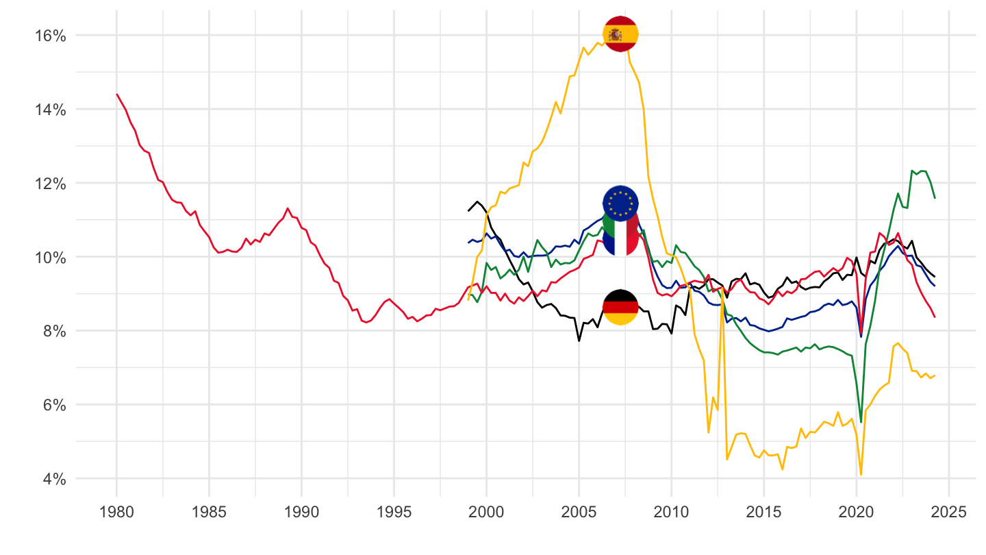
1999-
Code
nasq_10_ki %>%
  filter(geo %in% c("FR", "DE", "IT", "ES", "EA20"),
         na_item == "IRG_S14_S15",
         s_adj == "SCA") %>%
  quarter_to_date %>%
  mutate(values = values/100) %>%

  mutate(Geo = ifelse(geo == "EA20", "Europe", Geo)) %>%
  left_join(colors, by = c("Geo" = "country")) %>%
  filter(date >= as.Date("1999-01-01")) %>%
  ggplot + theme_minimal() + xlab("") + ylab("") +
  geom_line(aes(x = date, y = values, color = color)) +
  scale_color_identity() + add_5flags +
  scale_x_date(breaks = as.Date(paste0(seq(1940, 2100, 2), "-01-01")),
               labels = date_format("%Y")) +
  scale_y_continuous(breaks = 0.01*seq(0, 100, 2),
                labels = percent_format(a = 1))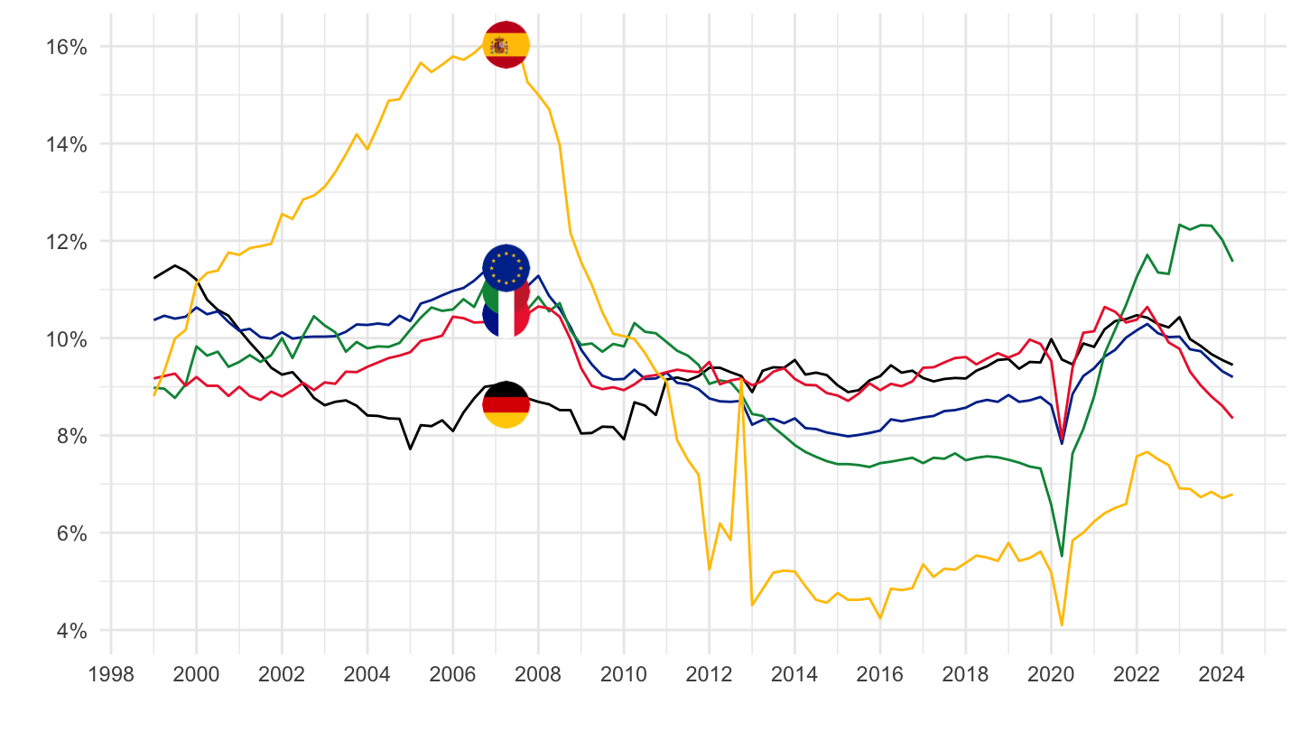
France, Germany, Eurozone
2015-
English
Code
nasq_10_ki %>%
  filter(geo %in% c("FR", "DE", "EA20"),
         na_item == "IRG_S14_S15",
         s_adj == "SCA") %>%
  quarter_to_date %>%
  mutate(values = values/100) %>%

  mutate(Geo = ifelse(geo == "EA20", "Europe", Geo)) %>%
  left_join(colors, by = c("Geo" = "country")) %>%
  filter(date >= as.Date("2015-01-01")) %>%
  ggplot + theme_minimal() + xlab("") + ylab("Gross investment rate of households") +
  geom_line(aes(x = date, y = values, color = color)) +
  scale_color_identity() + add_3flags +
  scale_x_date(breaks = as.Date(paste0(seq(1940, 2100, 1), "-01-01")),
               labels = date_format("%Y")) +
  scale_y_continuous(breaks = 0.01*seq(0, 100, .5),
                labels = percent_format(a = .1),)
French
Code
nasq_10_ki %>%
  filter(geo %in% c("FR", "DE", "EA20"),
         na_item == "IRG_S14_S15",
         s_adj == "SCA") %>%
  quarter_to_date %>%
  mutate(values = values/100) %>%

  mutate(Geo = ifelse(geo == "EA20", "Europe", Geo)) %>%
  left_join(colors, by = c("Geo" = "country")) %>%
  filter(date >= as.Date("2015-01-01")) %>%
  ggplot + theme_minimal() + xlab("") + ylab("Investissement brut des ménages") +
  geom_line(aes(x = date, y = values, color = color)) +
  scale_color_identity() + add_3flags +
  scale_x_date(breaks = as.Date(paste0(seq(1940, 2100, 1), "-01-01")),
               labels = date_format("%Y")) +
  scale_y_continuous(breaks = 0.01*seq(0, 100, .5),
                labels = percent_format(a = .1),)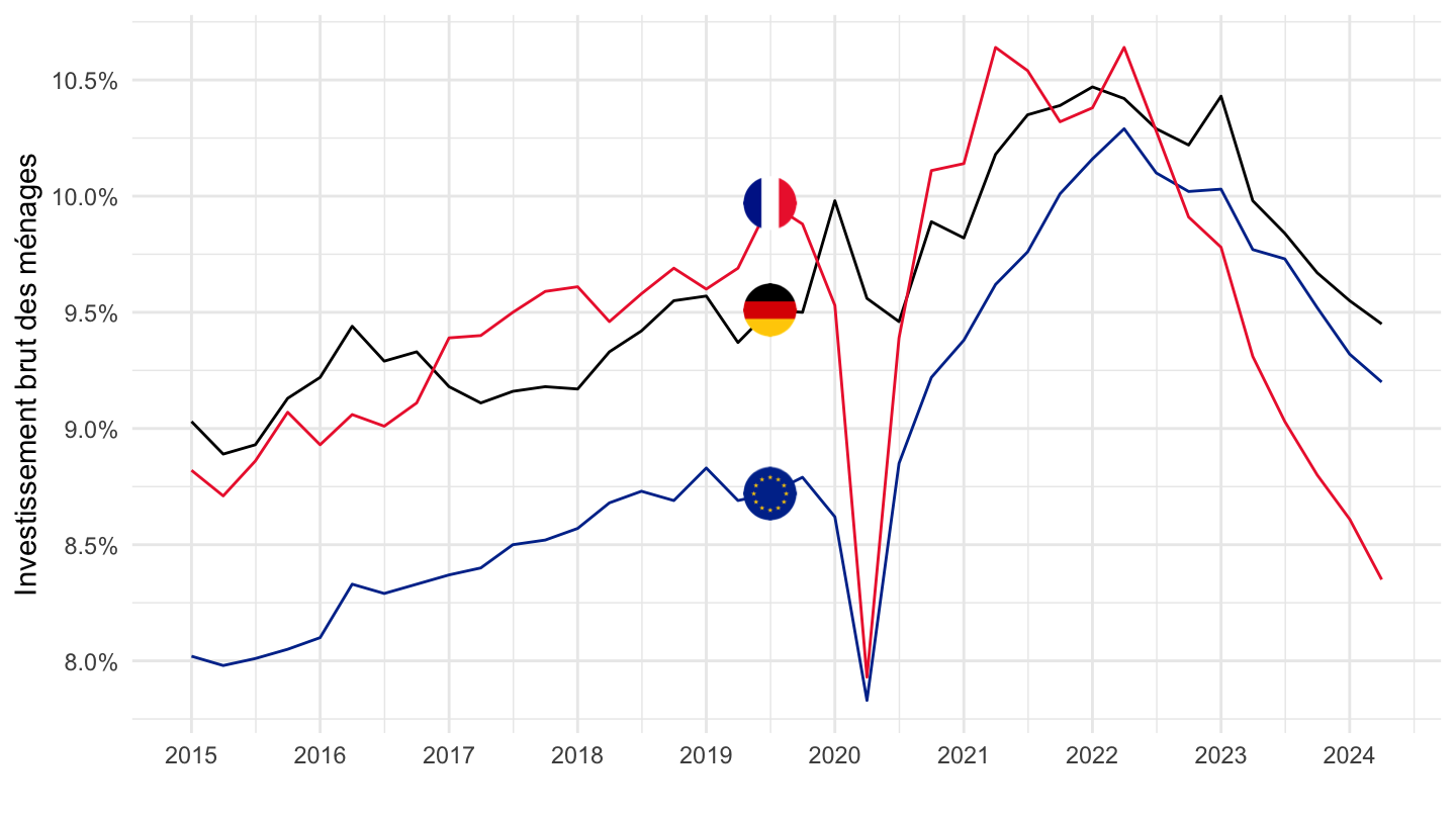
2019-
Code
nasq_10_ki %>%
  filter(geo %in% c("FR", "DE", "IT", "ES", "EA20"),
         na_item == "IRG_S14_S15",
         s_adj == "SCA") %>%
  quarter_to_date %>%
  mutate(values = values/100) %>%

  mutate(Geo = ifelse(geo == "EA20", "Europe", Geo)) %>%
  left_join(colors, by = c("Geo" = "country")) %>%
  filter(date >= as.Date("2019-01-01")) %>%
  ggplot + theme_minimal() + xlab("") + ylab("") +
  geom_line(aes(x = date, y = values, color = color)) +
  scale_color_identity() + add_5flags +
  scale_x_date(breaks = seq.Date(from = as.Date("2018-01-01"), to = as.Date("2100-01-01"), by = "3 months"),
               labels = date_format("%b %Y")) +
  theme(axis.text.x = element_text(angle = 45, vjust = 1, hjust = 1)) +
  scale_y_continuous(breaks = 0.01*seq(0, 100, 1),
                labels = percent_format(a = 1))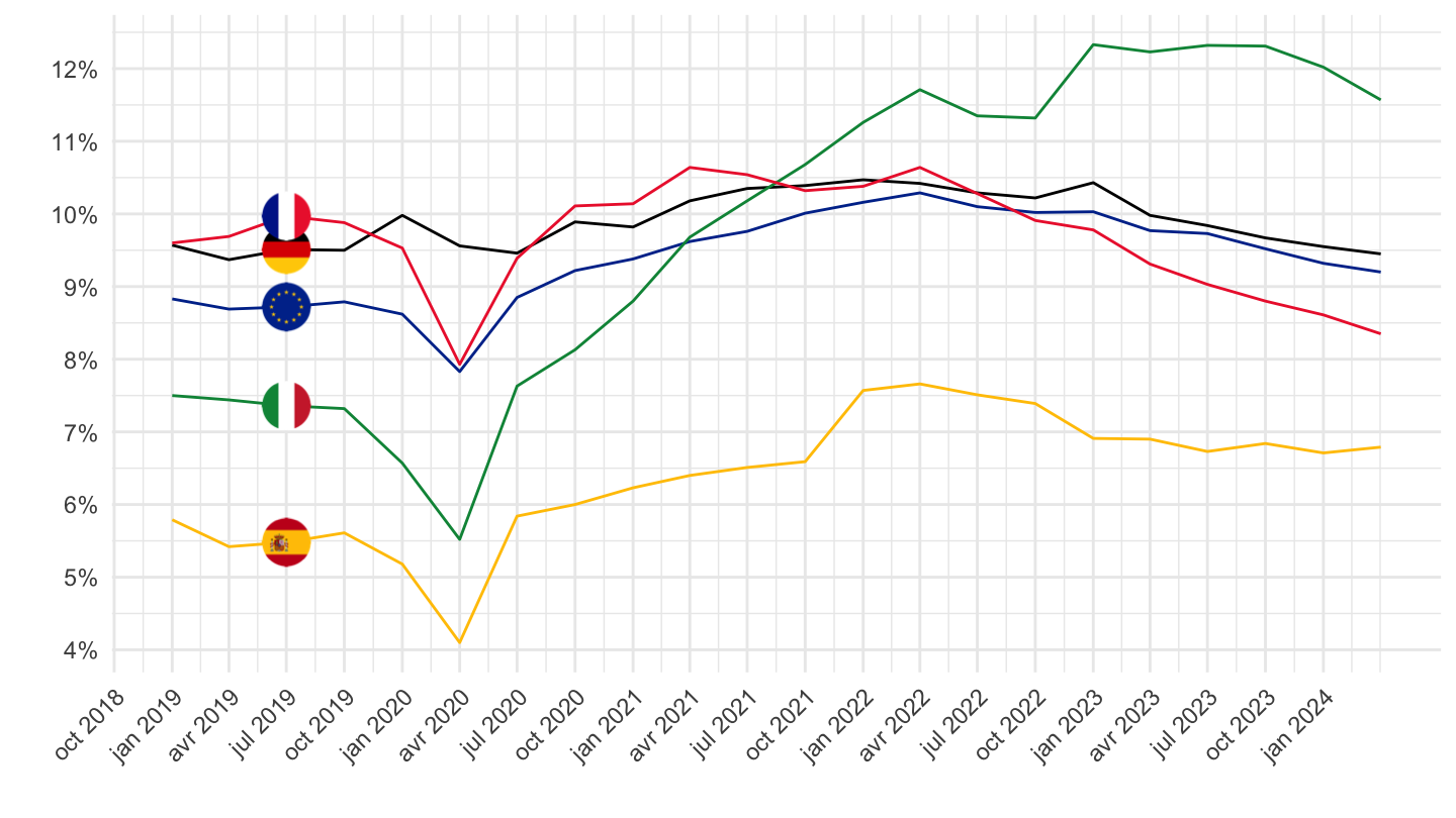
Gross investment rate of non-financial corporations (P51/B1G*100)
France, Germany, Spain, Italy, Europe
All
Code
nasq_10_ki %>%
  filter(geo %in% c("FR", "DE", "IT", "ES", "EA20"),
         na_item == "IRG_S11",
         s_adj == "SCA") %>%
  quarter_to_date %>%
  mutate(values = values/100) %>%

  mutate(Geo = ifelse(geo == "EA20", "Europe", Geo)) %>%
  left_join(colors, by = c("Geo" = "country")) %>%
  ggplot + theme_minimal() + xlab("") + ylab("") +
  geom_line(aes(x = date, y = values, color = color)) +
  scale_color_identity() + add_5flags +
  scale_x_date(breaks = as.Date(paste0(seq(1940, 2100, 5), "-01-01")),
               labels = date_format("%Y")) +
  scale_y_continuous(breaks = 0.01*seq(0, 100, 5),
                labels = percent_format(a = 1))
1999-
Code
nasq_10_ki %>%
  filter(geo %in% c("FR", "DE", "IT", "ES", "EA20"),
         na_item == "IRG_S11",
         s_adj == "SCA") %>%
  quarter_to_date %>%
  mutate(values = values/100) %>%

  mutate(Geo = ifelse(geo == "EA20", "Europe", Geo)) %>%
  left_join(colors, by = c("Geo" = "country")) %>%
  filter(date >= as.Date("1999-01-01")) %>%
  ggplot + theme_minimal() + xlab("") + ylab("") +
  geom_line(aes(x = date, y = values, color = color)) +
  scale_color_identity() + add_5flags +
  scale_x_date(breaks = as.Date(paste0(seq(1940, 2100, 2), "-01-01")),
               labels = date_format("%Y")) +
  scale_y_continuous(breaks = 0.01*seq(0, 100, 2),
                labels = percent_format(a = 1))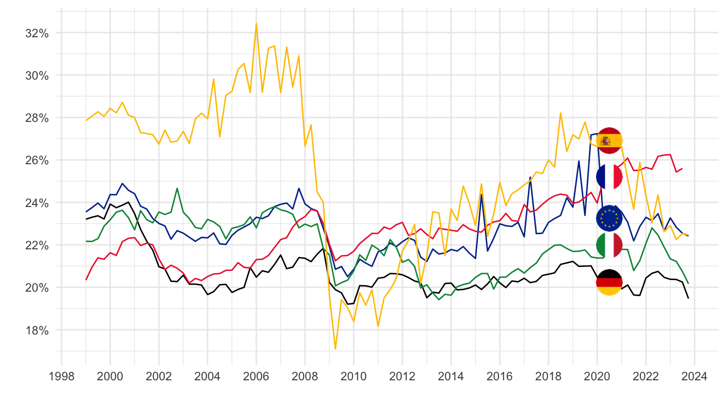
2015-
Code
nasq_10_ki %>%
  filter(geo %in% c("FR", "DE", "IT", "ES", "EA20"),
         na_item == "IRG_S11",
         s_adj == "SCA") %>%
  quarter_to_date %>%
  mutate(values = values/100) %>%

  mutate(Geo = ifelse(geo == "EA20", "Europe", Geo)) %>%
  left_join(colors, by = c("Geo" = "country")) %>%
  filter(date >= as.Date("2015-01-01")) %>%
  ggplot + theme_minimal() + xlab("") + ylab("") +
  geom_line(aes(x = date, y = values, color = color)) +
  scale_color_identity() + add_5flags +
  scale_x_date(breaks = as.Date(paste0(seq(1940, 2100, 1), "-01-01")),
               labels = date_format("%Y")) +
  scale_y_continuous(breaks = 0.01*seq(0, 100, 1),
                labels = percent_format(a = 1))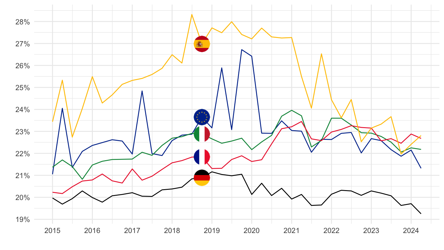
2019-
Code
nasq_10_ki %>%
  filter(geo %in% c("FR", "DE", "IT", "ES", "EA20"),
         na_item == "IRG_S11",
         s_adj == "SCA") %>%
  quarter_to_date %>%
  mutate(values = values/100) %>%

  mutate(Geo = ifelse(geo == "EA20", "Europe", Geo)) %>%
  left_join(colors, by = c("Geo" = "country")) %>%
  filter(date >= as.Date("2019-01-01")) %>%
  ggplot + theme_minimal() + xlab("") + ylab("") +
  geom_line(aes(x = date, y = values, color = color)) +
  scale_color_identity() + add_5flags +
  scale_x_date(breaks = seq.Date(from = as.Date("2018-01-01"), to = as.Date("2100-01-01"), by = "6 months"),
               labels = date_format("%b %Y")) +
  scale_y_continuous(breaks = 0.01*seq(0, 100, 1),
                labels = percent_format(a = 1))