
Last observation: 2026T2 (N = 1)
First observation: 2017T2 (N = 1)
Last data update: 21 oct. 2026, 07:14
Last compile: 22 oct. 2026, 09:14
`les-indices-de-salaire-de-base` |>
  group_by(sheets) |>
  summarise(Nobs = n()) |>
  arrange(-Nobs) |>
print_table_conditional()| sheets | Nobs |
|---|---|
| Sal. mens. ensemble | 36 |
`les-indices-de-salaire-de-base` |>
  group_by(TIME_PERIOD) |>
  summarise(Nobs = n()) |>
  arrange(desc(TIME_PERIOD)) |>
print_table_conditional()data1 <- `les-indices-de-salaire-de-base` |>
filter(secteur == "ENS",
sheets == "Sal. mens. ensemble") |>
select(TIME_PERIOD, value) |>
mutate(variable = "Salaire mensuel du secteur privé") |>
mutate(date = zoo::as.yearqtr(TIME_PERIOD, format = "%YT%q")) |>
filter(date >= zoo::as.yearqtr("2017 Q2")) |>
mutate(value = 100*value/value[1]) |>
ungroup()
data1 |>
ggplot() + geom_line(aes(x = date, y = value, color = variable)) +
theme_minimal() + xlab("") + ylab("") +
zoo::scale_x_yearqtr(labels = date_format("%YT%q"),
breaks = expand.grid(2017:2100, c(2, 4)) |>
mutate(breaks = zoo::as.yearqtr(paste0(Var1, "Q", Var2))) |>
pull(breaks)) +
scale_y_log10(breaks = seq(100, 200, 1)) +
theme(legend.position = c(0.2, 0.7),
legend.title = element_blank(),
axis.text.x = element_text(angle = 45, vjust = 1, hjust = 1)) +
geom_text(data = . %>%
filter(quarter(as.Date(date)) %in% c(2, 4)),
aes(x = date, y = value, label = round(value, 1)))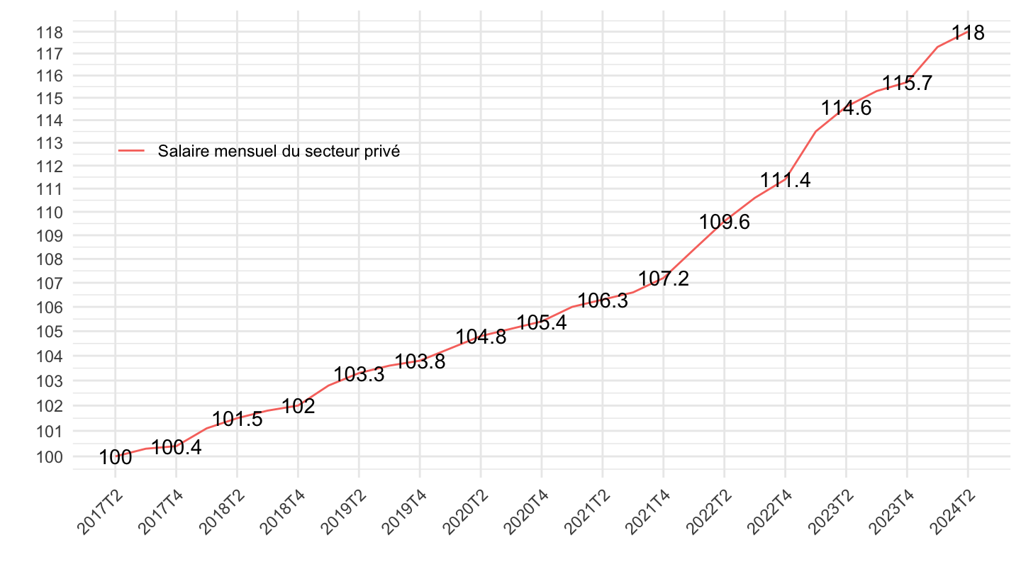
`IPCH-IPC-2025-ensemble` <- read_parquet(here::here("data", "insee", "IPCH-IPC-2025-ensemble.parquet"))
data2 <- `IPCH-IPC-2025-ensemble` |>
  filter(date >= as.Date("2017-06-01"),
         month(date) %in% c(3, 6, 9, 12)) |>
  group_by(INDICATEUR) |>
  mutate(value = 100*OBS_VALUE/OBS_VALUE[1]) |>
  transmute(TIME_PERIOD = paste0(year(date), "T", month(date)/3),
            value = 100*OBS_VALUE/OBS_VALUE[1],
            VARIABLE = INDICATEUR) |>
  mutate(variable = ifelse(VARIABLE == "IPC", "Prix Insee (IPC)", "Prix Eurostat (IPCH)")) |>
  mutate(date = zoo::as.yearqtr(TIME_PERIOD, format = "%YT%q")) |>
  ungroup()
data2 |>
  ggplot() + geom_line(aes(x = date, y = value, color = variable)) +
  theme_minimal() + xlab("") + ylab("") +
  zoo::scale_x_yearqtr(labels = date_format("%YT%q"),
                       breaks = expand.grid(2017:2100, c(2, 4)) |>
                         mutate(breaks = zoo::as.yearqtr(paste0(Var1, "Q", Var2))) |>
                         pull(breaks)) +
  scale_y_log10(breaks = seq(100, 200, 1)) +
  theme(legend.position = c(0.3, 0.9),
        legend.title = element_blank(),
        axis.text.x = element_text(angle = 45, vjust = 1, hjust = 1)) +
  geom_text(data = . %>%
              filter(quarter(as.Date(date)) %in% c(2, 4)),
            aes(x = date, y = value, label = round(value, 1)))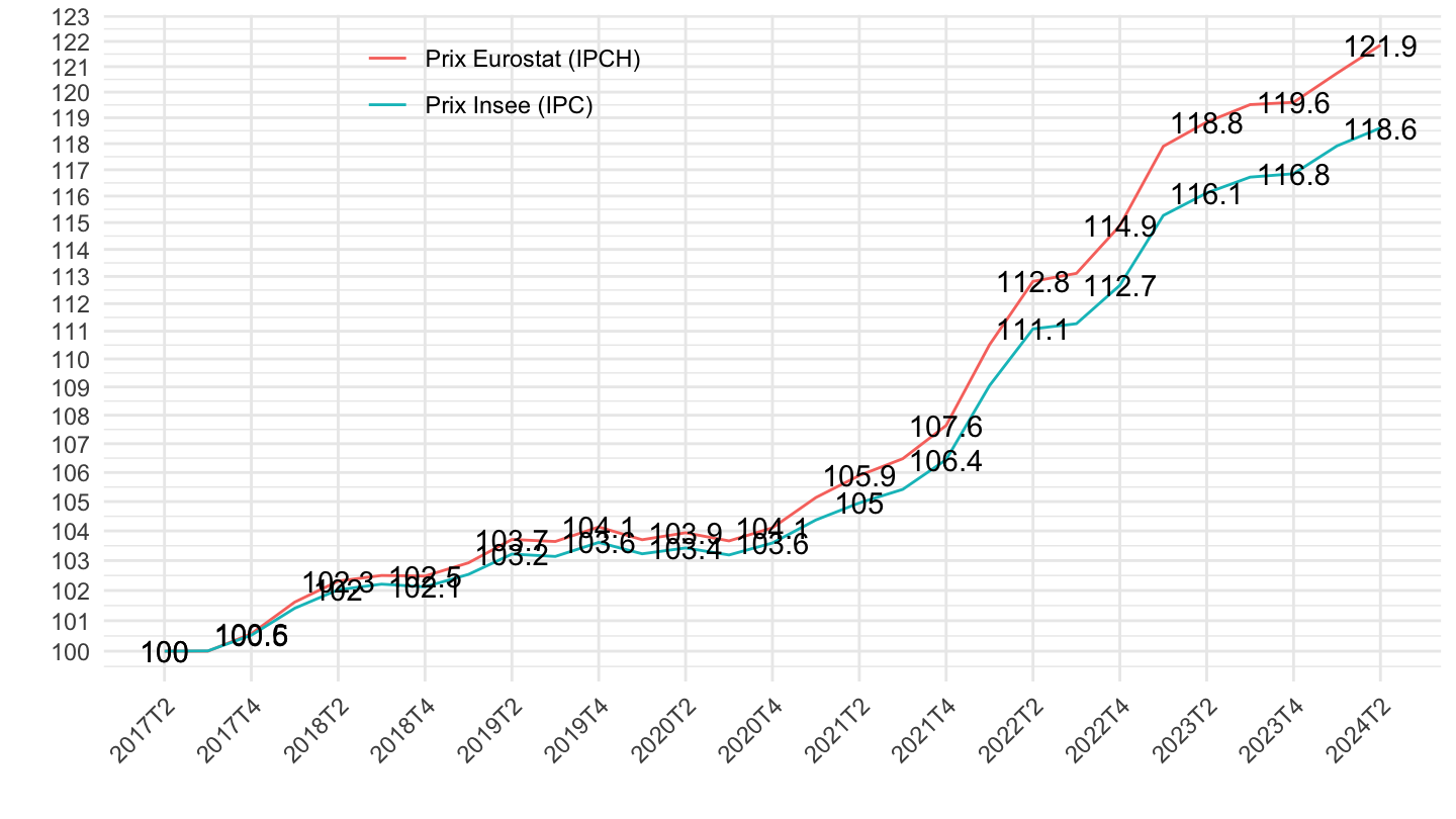
invisible(Sys.setlocale("LC_TIME", "fr_FR.UTF-8"))
data2 |>
  bind_rows(data1) |>
  ggplot() + geom_line(aes(x = date, y = value, color = variable)) +
  theme_minimal() + xlab("") + ylab("Augmentation depuis le 2017-T2") +
  zoo::scale_x_yearqtr(labels = date_format("%YT%q"),
                       breaks = expand.grid(2017:2100, c(2, 4)) |>
                         mutate(breaks = zoo::as.yearqtr(paste0(Var1, "Q", Var2))) |>
                         pull(breaks)) +
  scale_y_log10(breaks = seq(100, 200, 2),
                labels = percent(seq(100, 200, 2)/100-1)) +
  theme(legend.position = c(0.3, 0.8),
        legend.title = element_blank(),
        axis.text.x = element_text(angle = 45, vjust = 1, hjust = 1)) +
  geom_text_repel(data = . %>%
              filter(date == max(date)),
            aes(x = date, y = value, label = percent(value/100-1, acc = 0.1), color = variable)) +
  ggtitle("Augmentation des prix et des salaires depuis le 2ème trimestre 2017")
invisible(Sys.setlocale("LC_TIME", "fr_FR.UTF-8"))
data2 |>
  bind_rows(data1) |>
  filter(variable != "Prix Insee (IPC)") |>
  ggplot() + geom_line(aes(x = date, y = value, color = variable)) +
  theme_minimal() + xlab("") + ylab("Augmentation depuis le 2017-T2") +
  zoo::scale_x_yearqtr(labels = date_format("%YT%q"),
                       breaks = expand.grid(2017:2100, c(2, 4)) |>
                         mutate(breaks = zoo::as.yearqtr(paste0(Var1, "Q", Var2))) |>
                         pull(breaks)) +
  scale_y_log10(breaks = seq(100, 200, 2),
                labels = paste0("+", percent(seq(100, 200, 2)/100-1))) +
  theme(legend.position = c(0.3, 0.8),
        legend.title = element_blank(),
        axis.text.x = element_text(angle = 45, vjust = 1, hjust = 1)) +
  geom_label(data = . %>%
              filter(date == max(date)),
            aes(x = date, y = value, label = paste0("+", percent(value/100-1, acc = 0.1)), color = variable)) +
  ggtitle("Augmentation des prix et des salaires depuis le 2ème trimestre 2017")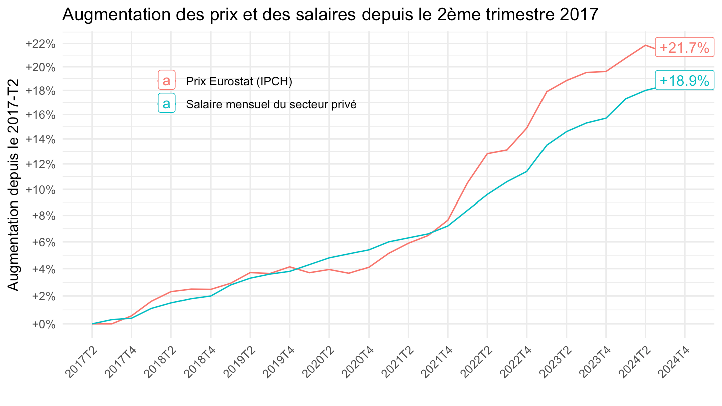
data1 <- `les-indices-de-salaire-de-base` |>
  filter(secteur == "ENS",
         sheets == "Sal. mens. ensemble") |>
  select(TIME_PERIOD, value) |>

  mutate(variable = "Salaire mensuel du secteur privé") |>
  mutate(date = zoo::as.yearqtr(TIME_PERIOD, format = "%YT%q")) |>
  filter(date >=  zoo::as.yearqtr("2017 Q4")) |>
  mutate(value = 100*value/value[1]) |>
  ungroup()
data1 |>
  ggplot() + geom_line(aes(x = date, y = value, color = variable)) +
  theme_minimal() + xlab("") + ylab("") +
  zoo::scale_x_yearqtr(labels = date_format("%YT%q"),
                       breaks = expand.grid(2017:2100, c(2, 4)) |>
                         mutate(breaks = zoo::as.yearqtr(paste0(Var1, "Q", Var2))) |>
                         pull(breaks)) +
  scale_y_log10(breaks = seq(100, 200, 1)) +
  theme(legend.position = c(0.2, 0.7),
        legend.title = element_blank(),
        axis.text.x = element_text(angle = 45, vjust = 1, hjust = 1)) +
  geom_text(data = . %>%
              filter(quarter(as.Date(date)) %in% c(2, 4)),
            aes(x = date, y = value, label = round(value, 1)))
`IPCH-IPC-2025-ensemble` <- read_parquet(here::here("data", "insee", "IPCH-IPC-2025-ensemble.parquet"))
data2 <- `IPCH-IPC-2025-ensemble` |>
  filter(date >= as.Date("2017-12-01"),
         month(date) %in% c(3, 6, 9, 12)) |>
  group_by(INDICATEUR) |>
  mutate(value = 100*OBS_VALUE/OBS_VALUE[1]) |>
  transmute(TIME_PERIOD = paste0(year(date), "T", month(date)/3),
            value = 100*OBS_VALUE/OBS_VALUE[1],
            VARIABLE = INDICATEUR) |>
  mutate(variable = ifelse(VARIABLE == "IPC", "Prix Insee (IPC)", "Prix Eurostat (IPCH)")) |>
  mutate(date = zoo::as.yearqtr(TIME_PERIOD, format = "%YT%q")) |>
  ungroup()
data2 |>
  ggplot() + geom_line(aes(x = date, y = value, color = variable)) +
  theme_minimal() + xlab("") + ylab("") +
  zoo::scale_x_yearqtr(labels = date_format("%YT%q"),
                       breaks = expand.grid(2017:2100, c(2, 4)) |>
                         mutate(breaks = zoo::as.yearqtr(paste0(Var1, "Q", Var2))) |>
                         pull(breaks)) +
  scale_y_log10(breaks = seq(100, 200, 1)) +
  theme(legend.position = c(0.3, 0.9),
        legend.title = element_blank(),
        axis.text.x = element_text(angle = 45, vjust = 1, hjust = 1)) +
  geom_text(data = . %>%
              filter(quarter(as.Date(date)) %in% c(2, 4)),
            aes(x = date, y = value, label = round(value, 1)))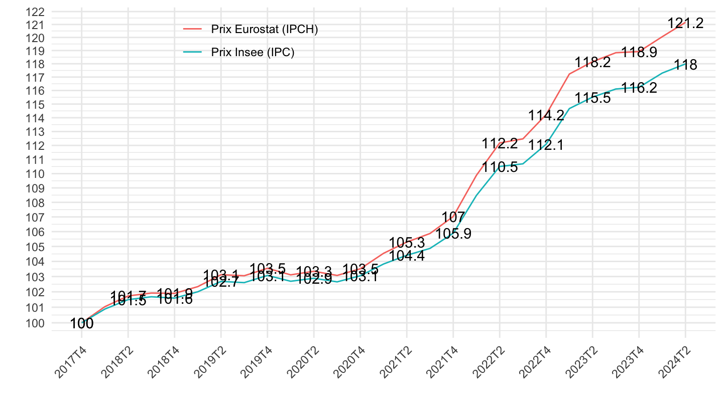
data2 |>
  bind_rows(data1) |>
  ggplot() + geom_line(aes(x = date, y = value, color = variable)) +
  theme_minimal() + xlab("") + ylab("") +
  zoo::scale_x_yearqtr(labels = date_format("%YT%q"),
                       breaks = expand.grid(2017:2100, c(2, 4)) |>
                         mutate(breaks = zoo::as.yearqtr(paste0(Var1, "Q", Var2))) |>
                         pull(breaks)) +
  scale_y_log10(breaks = seq(100, 200, 2)) +
  theme(legend.position = c(0.3, 0.9),
        legend.title = element_blank(),
        axis.text.x = element_text(angle = 45, vjust = 1, hjust = 1)) +
  geom_text(data = . %>%
              filter(date %in% zoo::as.yearqtr(c("2017 Q2", "2020 Q4", "2022 Q4", "2023 Q4"))),
            aes(x = date, y = value, label = round(value, 1)))
data1 <- `les-indices-de-salaire-de-base` |>
  filter(secteur == "ENS",
         sheets == "Sal. mens. ensemble") |>
  select(TIME_PERIOD, value) |>

  mutate(variable = "Salaire mensuel du secteur privé") |>
  mutate(date = zoo::as.yearqtr(TIME_PERIOD, format = "%YT%q")) |>
  filter(date >=  zoo::as.yearqtr("2019 Q4")) |>
  mutate(value = 100*value/value[1])
data1 |>
  ggplot() + geom_line(aes(x = date, y = value, color = variable)) +
  theme_minimal() + xlab("") + ylab("") +
  zoo::scale_x_yearqtr(labels = date_format("%YT%q"), n = 12) +
  scale_y_log10(breaks = seq(100, 200, 1)) +
  theme(legend.position = c(0.2, 0.7),
        legend.title = element_blank(),
        axis.text.x = element_text(angle = 45, vjust = 1, hjust = 1)) +
  geom_text(aes(x = date, y = value, label = round(value, 1)))
`IPCH-IPC-2025-ensemble` <- read_parquet(here::here("data", "insee", "IPCH-IPC-2025-ensemble.parquet"))

data2 <- `IPCH-IPC-2025-ensemble` |>
  filter(date >= as.Date("2019-12-01"),
         month(date) %in% c(3, 6, 9, 12)) |>
  group_by(INDICATEUR) |>
  mutate(value = 100*OBS_VALUE/OBS_VALUE[1]) |>
  transmute(TIME_PERIOD = paste0(year(date), "T", month(date)/3),
            value = 100*OBS_VALUE/OBS_VALUE[1],
            VARIABLE = INDICATEUR) |>
  mutate(variable = ifelse(VARIABLE == "IPC", "Prix Insee (IPC)", "Prix Eurostat (IPCH)")) |>
  mutate(date = zoo::as.yearqtr(TIME_PERIOD, format = "%YT%q"))

data2 |>
  ggplot() + geom_line(aes(x = date, y = value, color = variable)) +
  theme_minimal() + xlab("") + ylab("") +
  zoo::scale_x_yearqtr(labels = date_format("%YT%q"), n = 12) +
  scale_y_log10(breaks = seq(100, 200, 1)) +
  theme(legend.position = c(0.3, 0.9),
        legend.title = element_blank(),
        axis.text.x = element_text(angle = 45, vjust = 1, hjust = 1)) +
  geom_text(aes(x = date, y = value, label = round(value, 1)))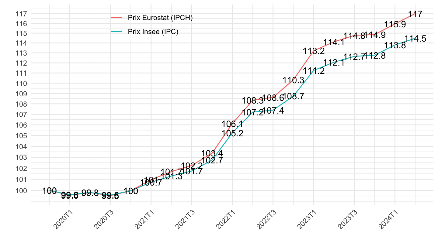
data2 |>
  bind_rows(data1) |>
  ggplot() + geom_line(aes(x = date, y = value, color = variable)) +
  theme_minimal() + xlab("") + ylab("") +
  zoo::scale_x_yearqtr(labels = date_format("%YT%q"), n = 24) +
  scale_y_log10(breaks = seq(100, 200, 1)) +
  theme(legend.position = c(0.3, 0.9),
        legend.title = element_blank(),
        axis.text.x = element_text(angle = 45, vjust = 1, hjust = 1)) +
  geom_text_repel(data = . %>% filter(date == max(date)), aes(x = date, y = value, label = round(value, 1), color = variable))
invisible(Sys.setlocale("LC_TIME", "fr_FR.UTF-8"))
data2 |>
  bind_rows(data1) |>
  filter(variable != "Prix Insee (IPC)") |>
  ggplot() + geom_line(aes(x = date, y = value, color = variable)) +
  theme_minimal() + xlab("") + ylab("Augmentation depuis le 2019-T4") +
  zoo::scale_x_yearqtr(labels = date_format("%YT%q"),
                       breaks = expand.grid(2019:2100, c(2, 4)) |>
                         mutate(breaks = zoo::as.yearqtr(paste0(Var1, "Q", Var2))) |>
                         pull(breaks)) +
  scale_y_log10(breaks = seq(100, 200, 2),
                labels = paste0("+", percent(seq(100, 200, 2)/100-1))) +
  theme(legend.position = c(0.3, 0.8),
        legend.title = element_blank(),
        axis.text.x = element_text(angle = 45, vjust = 1, hjust = 1)) +
  geom_label(data = . %>%
              filter(date == max(date)),
            aes(x = date, y = value, label = paste0("+", percent(value/100-1, acc = 0.1)), color = variable)) +
  ggtitle("Augmentation des prix et des salaires depuis le 4ème trimestre 2019")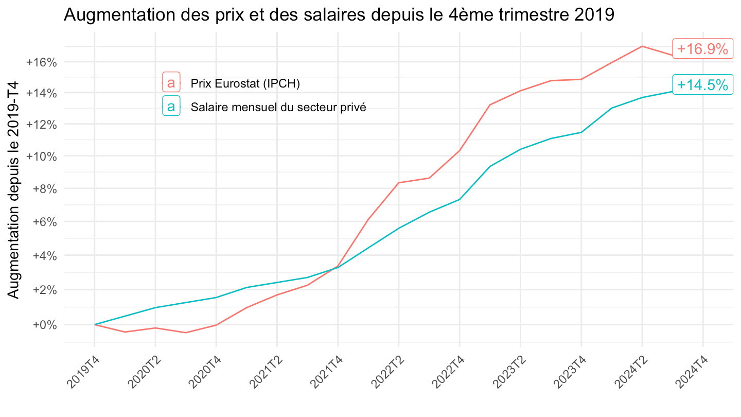
data1 <- `les-indices-de-salaire-de-base` |>
  filter(secteur == "ENS",
         sheets == "Sal. mens. ensemble") |>
  select(TIME_PERIOD, value) |>

  mutate(variable = "Salaire mensuel du secteur privé") |>
  mutate(date = zoo::as.yearqtr(TIME_PERIOD, format = "%YT%q")) |>
  filter(date >=  zoo::as.yearqtr("2020 Q4")) |>
  mutate(value = 100*value/value[1])
data1 |>
  ggplot() + geom_line(aes(x = date, y = value, color = variable)) +
  theme_minimal() + xlab("") + ylab("") +
  zoo::scale_x_yearqtr(labels = date_format("%YT%q"), n = 12) +
  scale_y_log10(breaks = seq(100, 200, 1)) +
  theme(legend.position = c(0.2, 0.7),
        legend.title = element_blank(),
        axis.text.x = element_text(angle = 45, vjust = 1, hjust = 1)) +
  geom_text(aes(x = date, y = value, label = round(value, 1)))
`IPCH-IPC-2025-ensemble` <- read_parquet(here::here("data", "insee", "IPCH-IPC-2025-ensemble.parquet"))
data2 <- `IPCH-IPC-2025-ensemble` |>
  filter(date >= as.Date("2020-12-01"),
         month(date) %in% c(3, 6, 9, 12)) |>
  group_by(INDICATEUR) |>
  mutate(value = 100*OBS_VALUE/OBS_VALUE[1]) |>
  transmute(TIME_PERIOD = paste0(year(date), "T", month(date)/3),
            value = 100*OBS_VALUE/OBS_VALUE[1],
            VARIABLE = INDICATEUR) |>
  mutate(variable = ifelse(VARIABLE == "IPC", "Prix Insee (IPC)", "Prix Eurostat (IPCH)")) |>
  mutate(date = zoo::as.yearqtr(TIME_PERIOD, format = "%YT%q"))
data2 |>
  ggplot() + geom_line(aes(x = date, y = value, color = variable)) +
  theme_minimal() + xlab("") + ylab("") +
  zoo::scale_x_yearqtr(labels = date_format("%YT%q"), n = 12) +
  scale_y_log10(breaks = seq(100, 200, 1)) +
  theme(legend.position = c(0.3, 0.9),
        legend.title = element_blank(),
        axis.text.x = element_text(angle = 45, vjust = 1, hjust = 1)) +
  geom_text(aes(x = date, y = value, label = round(value, 1)))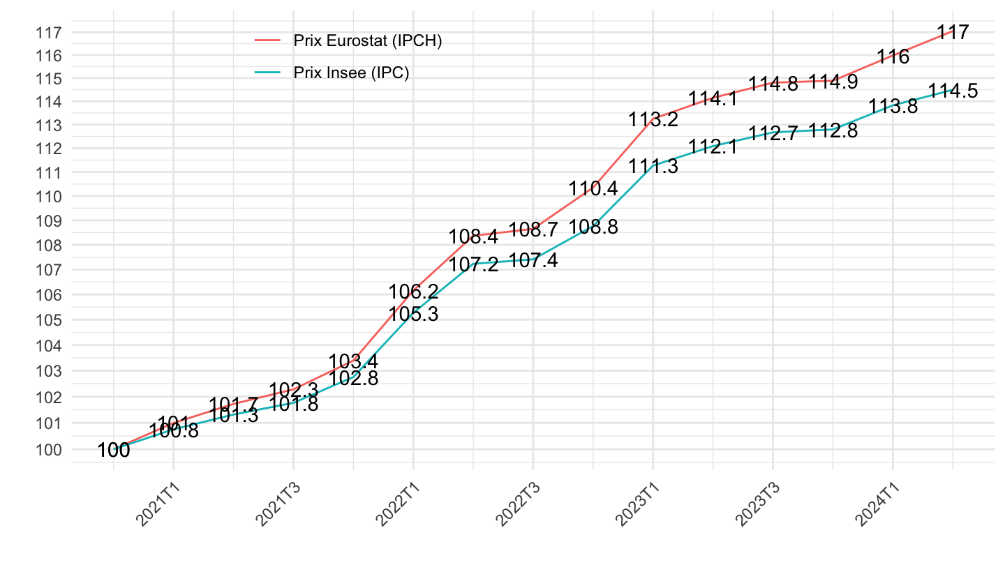
data_bind <- data2 |>
  bind_rows(data1) |>
  ungroup() |>
  select(date, value, variable) |>
  arrange(date)

# write_excel_csv(data_bind, file = "alter_eco_20230213.csv")

data_bind |>
  ggplot() + geom_line(aes(x = date, y = value, color = variable)) +
  theme_minimal() + xlab("") + ylab("Salaire de base") +
  zoo::scale_x_yearqtr(labels = date_format("%YT%q"),
                       breaks = seq(min(data_bind$date), max(data_bind$date), by = 0.25)) +
  scale_y_log10(breaks = seq(100, 200, 1)) +
  theme(legend.position = c(0.3, 0.9),
        legend.title = element_blank(),
        axis.text.x = element_text(angle = 45, vjust = 1, hjust = 1)) +
  geom_label(data = . %>%
              filter(date == max(date)),
            aes(x = date, y = value, label = round(value, 1)))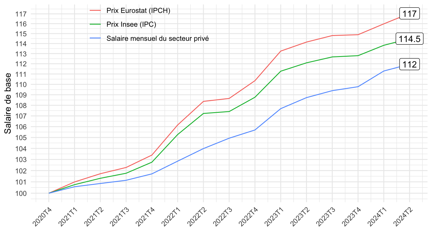
data1 <- `les-indices-de-salaire-de-base` |>
  filter(secteur == "ENS",
         sheets == "Sal. mens. ensemble") |>
  select(TIME_PERIOD, value) |>

  mutate(variable = "Salaire mensuel du secteur privé") |>
  mutate(date = zoo::as.yearqtr(TIME_PERIOD, format = "%YT%q")) |>
  filter(date >=  zoo::as.yearqtr("2021 Q1")) |>
  mutate(value = 100*value/value[1])
data1 |>
  ggplot() + geom_line(aes(x = date, y = value, color = variable)) +
  theme_minimal() + xlab("") + ylab("") +
  zoo::scale_x_yearqtr(labels = date_format("%YT%q"), n = 12) +
  scale_y_log10(breaks = seq(100, 200, 1)) +
  theme(legend.position = c(0.2, 0.7),
        legend.title = element_blank(),
        axis.text.x = element_text(angle = 45, vjust = 1, hjust = 1)) +
  geom_text(aes(x = date, y = value, label = round(value, 1)))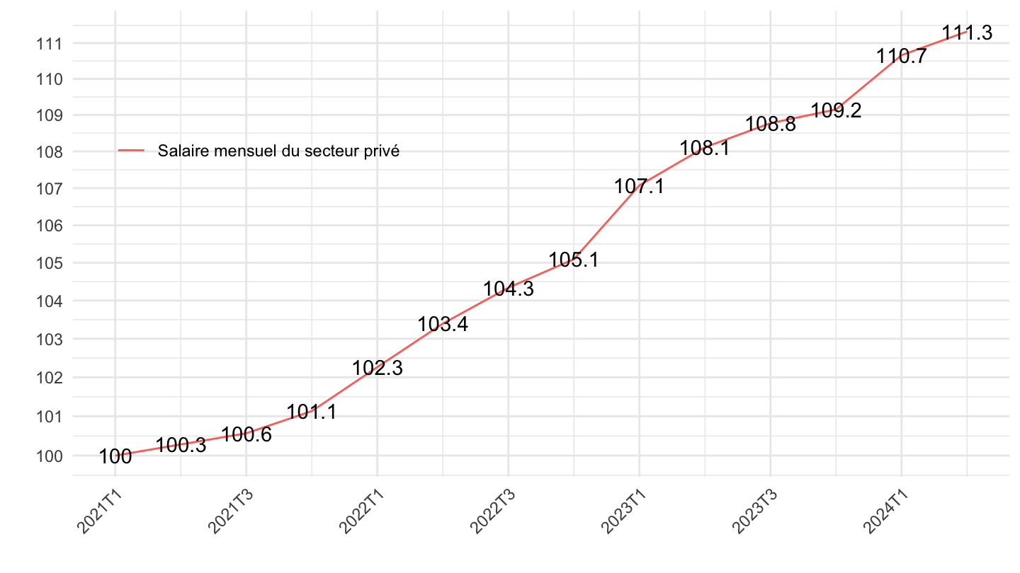
`IPCH-IPC-2025-ensemble` <- read_parquet(here::here("data", "insee", "IPCH-IPC-2025-ensemble.parquet"))
data2 <- `IPCH-IPC-2025-ensemble` |>
  filter(date >= as.Date("2021-03-01"),
         month(date) %in% c(3, 6, 9, 12)) |>
  group_by(INDICATEUR) |>
  mutate(value = 100*OBS_VALUE/OBS_VALUE[1]) |>
  transmute(TIME_PERIOD = paste0(year(date), "T", month(date)/3),
            value = 100*OBS_VALUE/OBS_VALUE[1],
            VARIABLE = INDICATEUR) |>
  mutate(variable = ifelse(VARIABLE == "IPC", "Prix Insee (IPC)", "Prix Eurostat (IPCH)")) |>
  mutate(date = zoo::as.yearqtr(TIME_PERIOD, format = "%YT%q"))
data2 |>
  ggplot() + geom_line(aes(x = date, y = value, color = variable)) +
  theme_minimal() + xlab("") + ylab("") +
  zoo::scale_x_yearqtr(labels = date_format("%YT%q"), n = 12) +
  scale_y_log10(breaks = seq(100, 200, 1)) +
  theme(legend.position = c(0.3, 0.9),
        legend.title = element_blank(),
        axis.text.x = element_text(angle = 45, vjust = 1, hjust = 1)) +
  geom_text(aes(x = date, y = value, label = round(value, 1)))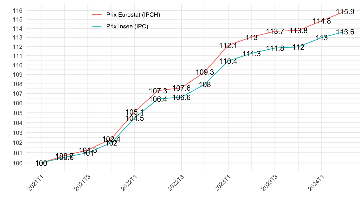
data_bind <- data2 |>
  bind_rows(data1) |>
  ungroup() |>
  select(date, value, variable) |>
  arrange(date)

# write_excel_csv(data_bind, file = "alter_eco_20230213.csv")

data_bind |>
  ggplot() + geom_line(aes(x = date, y = value, color = variable)) +
  theme_minimal() + xlab("") + ylab("") +
  zoo::scale_x_yearqtr(labels = date_format("%YT%q"), n = 12) +
  scale_y_log10(breaks = seq(100, 200, 1)) +
  theme(legend.position = c(0.3, 0.9),
        legend.title = element_blank(),
        axis.text.x = element_text(angle = 45, vjust = 1, hjust = 1)) +
  geom_text(aes(x = date, y = value, label = round(value, 1)))
data1 <- `les-indices-de-salaire-de-base` |>
  filter(secteur == "ENS",
         sheets == "Sal. mens. ensemble") |>
  select(TIME_PERIOD, value) |>

  mutate(variable = "Salaire mensuel du secteur privé") |>
  mutate(date = zoo::as.yearqtr(TIME_PERIOD, format = "%YT%q")) |>
  filter(date >=  zoo::as.yearqtr("2021 Q2")) |>
  mutate(value = 100*value/value[1])


data1 |>
  ggplot() + geom_line(aes(x = date, y = value, color = variable)) +
  theme_minimal() + xlab("") + ylab("") +
  zoo::scale_x_yearqtr(labels = date_format("%YT%q"), n = 12) +
  scale_y_log10(breaks = seq(100, 200, 1)) +
  theme(legend.position = c(0.2, 0.7),
        legend.title = element_blank(),
        axis.text.x = element_text(angle = 45, vjust = 1, hjust = 1)) +
  geom_text(aes(x = date, y = value, label = round(value, 1)))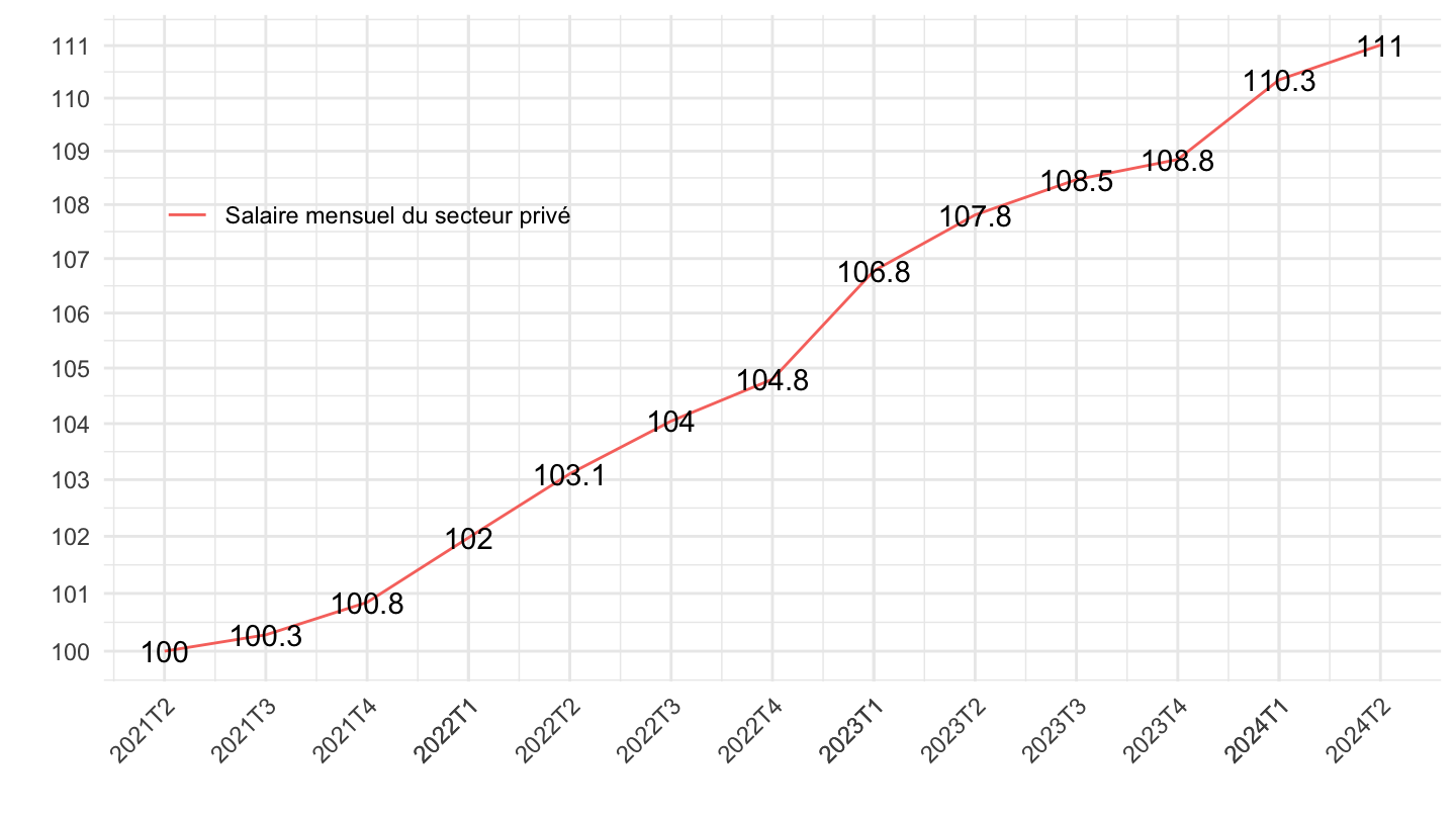
`IPCH-IPC-2025-ensemble` <- read_parquet(here::here("data", "insee", "IPCH-IPC-2025-ensemble.parquet"))
data2 <- `IPCH-IPC-2025-ensemble` |>
  filter(date >= as.Date("2021-06-01"),
         month(date) %in% c(3, 6, 9, 12)) |>
  group_by(INDICATEUR) |>
  mutate(value = 100*OBS_VALUE/OBS_VALUE[1]) |>
  transmute(TIME_PERIOD = paste0(year(date), "T", month(date)/3),
            value = 100*OBS_VALUE/OBS_VALUE[1],
            VARIABLE = INDICATEUR) |>
  mutate(variable = ifelse(VARIABLE == "IPC", "Prix Insee (IPC)", "Prix Eurostat (IPCH)")) |>
  mutate(date = zoo::as.yearqtr(TIME_PERIOD, format = "%YT%q"))
data2 |>
  ggplot() + geom_line(aes(x = date, y = value, color = variable)) +
  theme_minimal() + xlab("") + ylab("") +
  zoo::scale_x_yearqtr(labels = date_format("%YT%q"), n = 12) +
  scale_y_log10(breaks = seq(100, 200, 1)) +
  theme(legend.position = c(0.3, 0.9),
        legend.title = element_blank(),
        axis.text.x = element_text(angle = 45, vjust = 1, hjust = 1)) +
  geom_text(aes(x = date, y = value, label = round(value, 1)))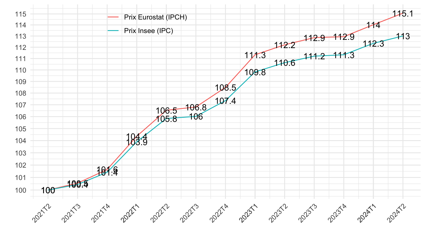
data_bind <- data2 |>
  bind_rows(data1) |>
  ungroup() |>
  select(date, value, variable) |>
  arrange(date)

# write_excel_csv(data_bind, file = "alter_eco_20230213.csv")

data_bind |>
  ggplot() + geom_line(aes(x = date, y = value, color = variable)) +
  theme_minimal() + xlab("") + ylab("Hausse vs. 2ème trimestre 2021") +
  zoo::scale_x_yearqtr(labels = date_format("%YT%q"),
                       breaks = expand.grid(2021:2100, c(1, 2, 3, 4)) |>
                         mutate(breaks = zoo::as.yearqtr(paste0(Var1, "Q", Var2))) |>
                         pull(breaks)) +
  scale_y_log10(breaks = seq(100, 200, 1)) +
  theme(legend.position = c(0.3, 0.9),
        legend.title = element_blank(),
        axis.text.x = element_text(angle = 45, vjust = 1, hjust = 1)) +
  geom_label(data = . %>% filter(date == max(date)), aes(x = date, y = value, label = round(value, 1), color = variable))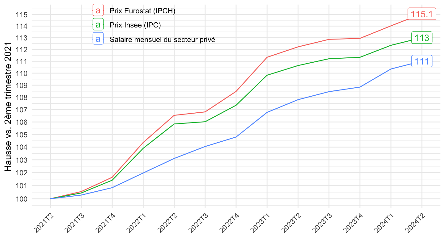
data1 <- `les-indices-de-salaire-de-base` |>
  filter(secteur == "ENS",
         sheets == "Sal. mens. ensemble") |>
  select(TIME_PERIOD, value) |>

  mutate(variable = "Salaire mensuel du secteur privé") |>
  mutate(date = zoo::as.yearqtr(TIME_PERIOD, format = "%YT%q")) |>
  filter(date >=  zoo::as.yearqtr("2021 Q4")) |>
  mutate(value = 100*value/value[1])


data1 |>
  ggplot() + geom_line(aes(x = date, y = value, color = variable)) +
  theme_minimal() + xlab("") + ylab("") +
  zoo::scale_x_yearqtr(labels = date_format("%YT%q"), n = 12) +
  scale_y_log10(breaks = seq(100, 200, 1)) +
  theme(legend.position = c(0.2, 0.7),
        legend.title = element_blank(),
        axis.text.x = element_text(angle = 45, vjust = 1, hjust = 1)) +
  geom_text(aes(x = date, y = value, label = round(value, 1)))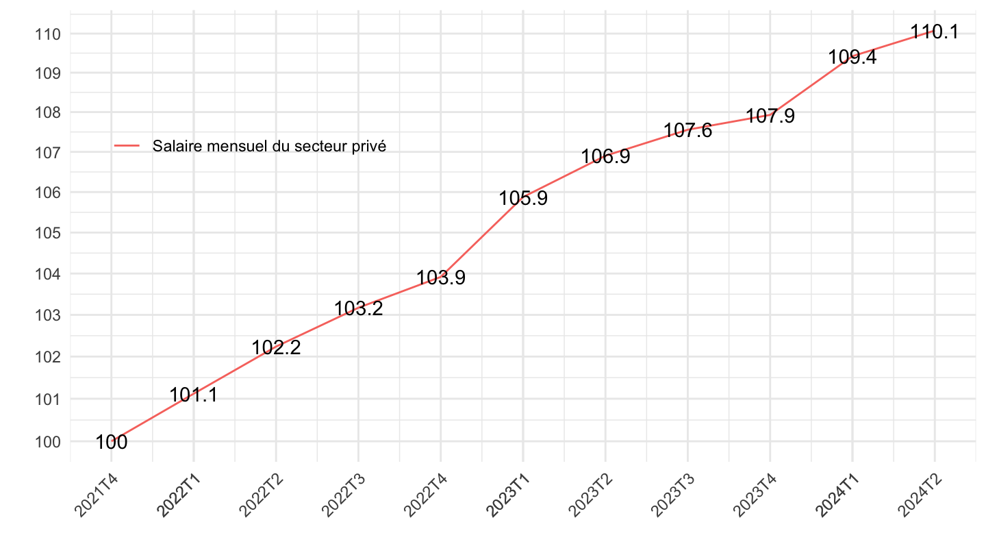
`IPCH-IPC-2025-ensemble` <- read_parquet(here::here("data", "insee", "IPCH-IPC-2025-ensemble.parquet"))
data2 <- `IPCH-IPC-2025-ensemble` |>
  filter(date >= as.Date("2021-12-01"),
         month(date) %in% c(3, 6, 9, 12)) |>
  group_by(INDICATEUR) |>
  mutate(value = 100*OBS_VALUE/OBS_VALUE[1]) |>
  transmute(TIME_PERIOD = paste0(year(date), "T", month(date)/3),
            value = 100*OBS_VALUE/OBS_VALUE[1],
            VARIABLE = INDICATEUR) |>
  mutate(variable = ifelse(VARIABLE == "IPC", "Prix Insee (IPC)", "Prix Eurostat (IPCH)")) |>
  mutate(date = zoo::as.yearqtr(TIME_PERIOD, format = "%YT%q"))
data2 |>
  ggplot() + geom_line(aes(x = date, y = value, color = variable)) +
  theme_minimal() + xlab("") + ylab("") +
  zoo::scale_x_yearqtr(labels = date_format("%YT%q"), n = 12) +
  scale_y_log10(breaks = seq(100, 200, 1)) +
  theme(legend.position = c(0.3, 0.9),
        legend.title = element_blank(),
        axis.text.x = element_text(angle = 45, vjust = 1, hjust = 1)) +
  geom_text(aes(x = date, y = value, label = round(value, 1)))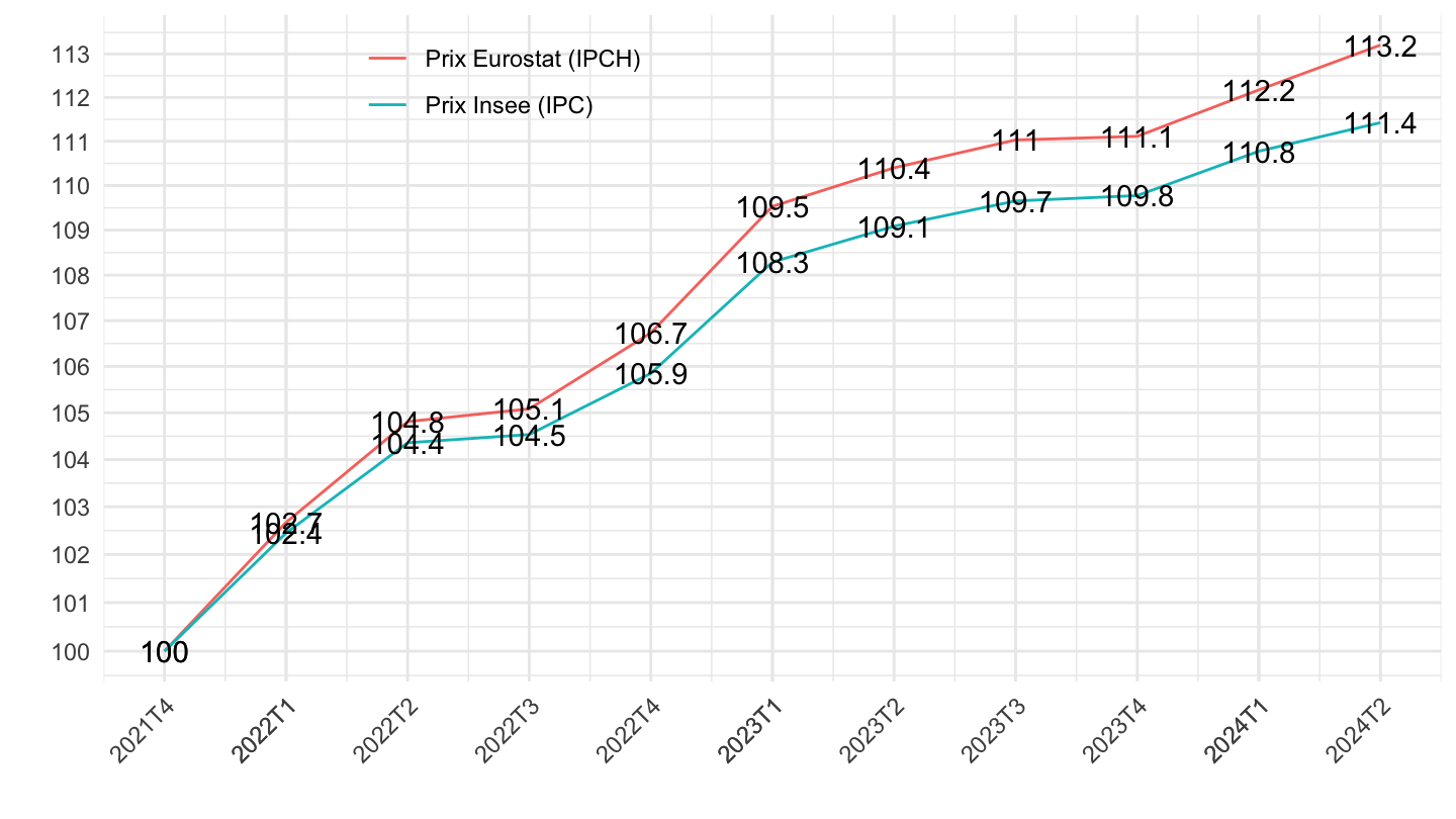
data_bind <- data2 |>
  bind_rows(data1) |>
  ungroup() |>
  select(date, value, variable) |>
  arrange(date)

# write_excel_csv(data_bind, file = "alter_eco_20230213.csv")

data_bind |>
  ggplot() + geom_line(aes(x = date, y = value, color = variable)) +
  theme_minimal() + xlab("") + ylab("") +
  zoo::scale_x_yearqtr(labels = date_format("%YT%q"),
                       breaks = expand.grid(2021:2100, c(1, 2, 3, 4)) |>
                         mutate(breaks = zoo::as.yearqtr(paste0(Var1, "Q", Var2))) |>
                         pull(breaks)) +
  scale_y_log10(breaks = seq(100, 200, 1)) +
  theme(legend.position = c(0.3, 0.9),
        legend.title = element_blank(),
        axis.text.x = element_text(angle = 45, vjust = 1, hjust = 1)) +
  geom_text(aes(x = date, y = value, label = round(value, 1)))
data_bind <- data2 |>
  bind_rows(data1) |>
  ungroup() |>
  select(date, value, variable) |>
  arrange(date)

# write_excel_csv(data_bind, file = "alter_eco_20230213.csv")

data_bind |>
  ggplot() + geom_line(aes(x = date, y = value, color = variable)) +
  theme_minimal() + xlab("") + ylab("") +
  zoo::scale_x_yearqtr(labels = date_format("%YT%q"),
                       breaks = expand.grid(2021:2100, c(1, 2, 3, 4)) |>
                         mutate(breaks = zoo::as.yearqtr(paste0(Var1, "Q", Var2))) |>
                         pull(breaks)) +
  scale_y_log10(breaks = seq(100, 200, 1)) +
  theme(legend.position = c(0.3, 0.9),
        legend.title = element_blank(),
        axis.text.x = element_text(angle = 45, vjust = 1, hjust = 1)) +
  geom_label_repel(data = . %>%
              filter(date == max(date)),
            aes(x = date, y = value, label = sprintf("%+.1f%%", value-100), color = variable)) +
  ggtitle("Augmentation des prix et des salaires sur 3 ans depuis le 4ème trimestre 2021")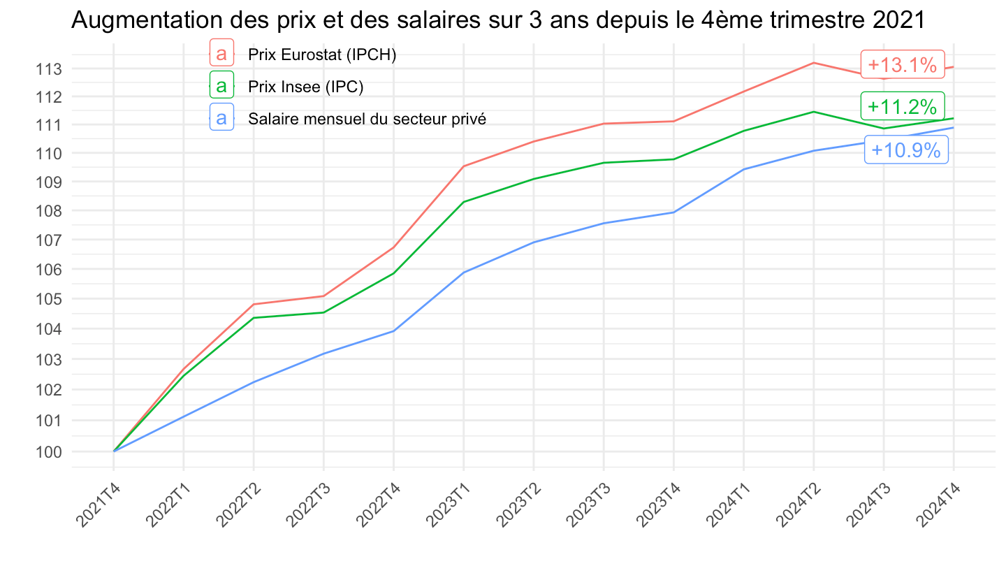
`les-indices-de-salaire-de-base` |>
  filter(secteur == "ENS") |>
  mutate(date = zoo::as.yearqtr(TIME_PERIOD, format = "%YT%q")) |>
  ggplot() + geom_line(aes(x = date, y = value, color = sheets)) +
  theme_minimal() + xlab("") + ylab("") +
  zoo::scale_x_yearqtr(labels = date_format("%YT%q"), n = 24) +
  scale_y_log10(breaks = seq(100, 200, 2)) +
  theme(legend.position = c(0.2, 0.7),
        legend.title = element_blank(),
        axis.text.x = element_text(angle = 45, vjust = 1, hjust = 1))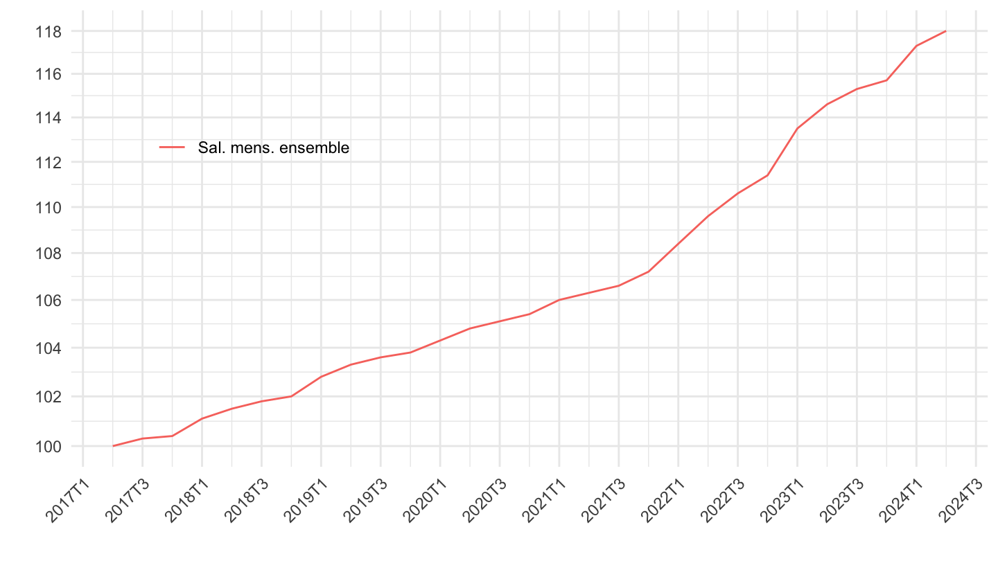
`les-indices-de-salaire-de-base` |>
  filter(secteur == "ENS") |>
  mutate(date = zoo::as.yearqtr(TIME_PERIOD, format = "%YT%q")) |>
  filter(date >=  zoo::as.yearqtr("2019 Q4")) |>
  group_by(sheets) |>
  mutate(value = 100*value/value[1]) |>
  ggplot() + geom_line(aes(x = date, y = value, color = sheets)) +
  theme_minimal() + xlab("") + ylab("") +
  zoo::scale_x_yearqtr(labels = date_format("%YT%q"), n = 24) +
  scale_y_log10(breaks = seq(100, 200, 1)) +
  theme(legend.position = c(0.2, 0.7),
        legend.title = element_blank(),
        axis.text.x = element_text(angle = 45, vjust = 1, hjust = 1))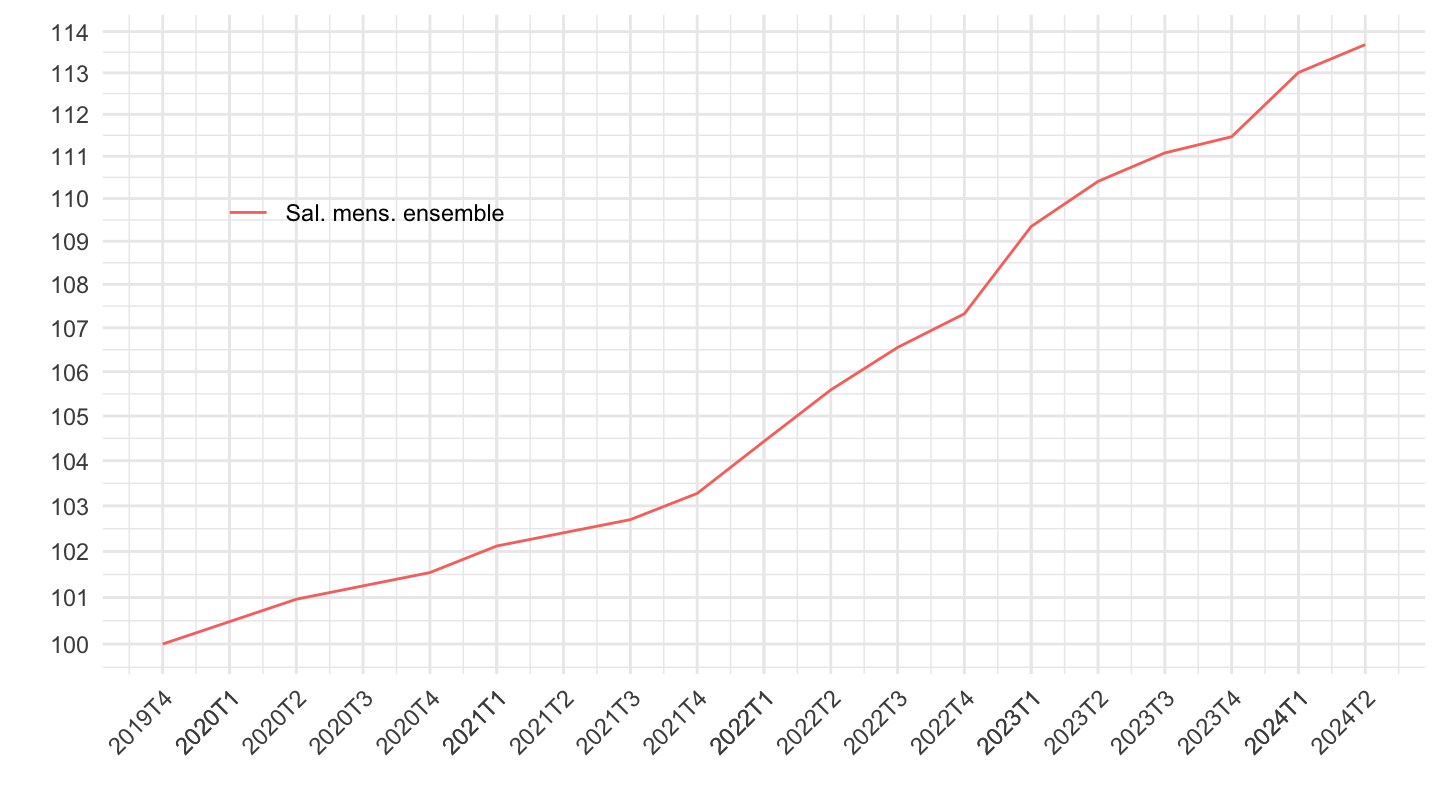
`les-indices-de-salaire-de-base` |>
  filter(secteur == "ENS") |>
  mutate(date = zoo::as.yearqtr(TIME_PERIOD, format = "%YT%q")) |>
  filter(date >=  zoo::as.yearqtr("2021 Q3")) |>
  group_by(sheets) |>
  mutate(value = 100*value/value[1]) |>
  ggplot() + geom_line(aes(x = date, y = value, color = sheets)) +
  theme_minimal() + xlab("") + ylab("") +
  zoo::scale_x_yearqtr(labels = date_format("%YT%q"), n = 12) +
  scale_y_log10(breaks = seq(100, 200, 1)) +
  theme(legend.position = c(0.2, 0.7),
        legend.title = element_blank(),
        axis.text.x = element_text(angle = 45, vjust = 1, hjust = 1))
`les-indices-de-salaire-de-base` |>
  filter(secteur == "ENS") |>
  mutate(date = zoo::as.yearqtr(TIME_PERIOD, format = "%YT%q")) |>
  filter(date >=  zoo::as.yearqtr("2020 Q4")) |>
  group_by(sheets) |>
  mutate(value = 100*value/value[1]) |>
  ggplot() + geom_line(aes(x = date, y = value, color = sheets)) +
  theme_minimal() + xlab("") + ylab("") +
  zoo::scale_x_yearqtr(labels = date_format("%YT%q"), n = 12) +
  scale_y_log10(breaks = seq(100, 200, 1)) +
  theme(legend.position = c(0.2, 0.7),
        legend.title = element_blank(),
        axis.text.x = element_text(angle = 45, vjust = 1, hjust = 1))