Family Database - FAMILY
Data - OECD
Info
Données sur la demographie
| source | dataset | .html | .RData |
|---|---|---|---|
| 2024-09-14 | 2024-09-14 | ||
| 2024-06-20 | 2022-01-31 | ||
| 2024-06-20 | 2023-10-10 | ||
| 2024-06-20 | 2021-12-18 | ||
| 2024-09-14 | 2024-09-14 | ||
| 2024-09-14 | 2024-09-14 | ||
| 2024-09-11 | 2024-02-13 |
Last
Code
FAMILY %>%
  group_by(obsTime) %>%
  summarise(Nobs = n()) %>%
  arrange(desc(obsTime)) %>%
  head(1) %>%
print_table_conditional()| obsTime | Nobs |
|---|---|
| 2022 | 522 |
COU
Code
FAMILY %>%
  left_join(FAMILY_var$COU, by = "COU") %>%
  group_by(COU, Cou) %>%
  summarise(Nobs = n()) %>%
  arrange(-Nobs) %>%
  mutate(Flag = gsub(" ", "-", str_to_lower(Cou)),
         Flag = paste0('<img src="../../icon/flag/vsmall/', Flag, '.png" alt="Flag">')) %>%
  select(Flag, everything()) %>%
  {if (is_html_output()) datatable(., filter = 'top', rownames = F, escape = F) else .}
SEX
Code
FAMILY %>%
  left_join(FAMILY_var$SEX, by = "SEX") %>%
  group_by(SEX, Sex) %>%
  summarise(Nobs = n()) %>%
  arrange(-Nobs) %>%
print_table_conditional()| SEX | Sex | Nobs |
|---|---|---|
| TOTAL | Total | 42900 |
| MALE | Male | 3914 |
| FEMALE | Female | 3910 |
IND
Code
FAMILY %>%
  left_join(FAMILY_var$IND, by = "IND") %>%
  group_by(IND, Ind) %>%
  summarise(Nobs = n()) %>%
  arrange(-Nobs) %>%
  print_table_conditional()
obsTime
Code
FAMILY %>%
  group_by(obsTime) %>%
  summarise(Nobs = n()) %>%
  arrange(desc(obsTime)) %>%
  print_table_conditional()
Total fertility rate - FAM1
Table
Code
FAMILY %>%
  filter(IND == "FAM1") %>%
  left_join(FAMILY_var$COU, by = "COU") %>%
  group_by(COU, Cou) %>%
  summarise(Nobs = n(),
            obsTime = last(obsTime),
            obsValue = last(obsValue)) %>%
  mutate(Flag = gsub(" ", "-", str_to_lower(Cou)),
         Flag = paste0('<img src="../../icon/flag/vsmall/', Flag, '.png" alt="Flag">')) %>%
  select(Flag, everything()) %>%
  {if (is_html_output()) datatable(., filter = 'top', rownames = F, escape = F) else .}
France, Italy, Germany
Code
FAMILY %>%
  filter(IND == "FAM1",
         COU %in% c("FRA", "DEU", "ITA")) %>%
  year_to_date() %>%
  left_join(FAMILY_var$COU, by = "COU") %>%
  rename(Location = Cou) %>%
  left_join(colors, by = c("Location" = "country")) %>%
  ggplot(.) + theme_minimal() + scale_color_identity() +
  geom_line(aes(x = date, y = obsValue, color = color)) +
  xlab("") + ylab("") + add_3flags +
  scale_x_date(breaks = seq(1940, 2050, 5) %>% paste0("-01-01") %>% as.Date,
               labels = date_format("%Y")) +
  scale_y_continuous(breaks = seq(0, 10, 0.2))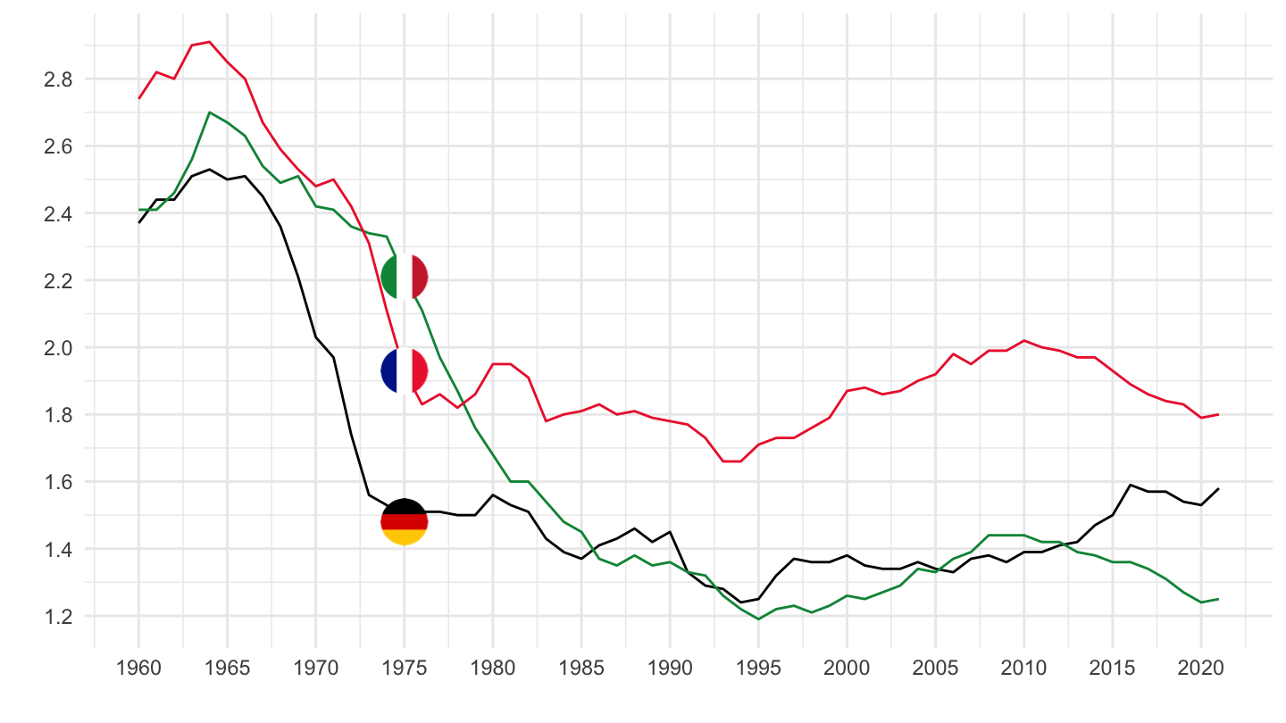
Crude marriage rate (marriages per 1000 people) - FAM4A
Table
Code
FAMILY %>%
  filter(IND == "FAM4A") %>%
  left_join(FAMILY_var$COU, by = "COU") %>%
  group_by(COU, Cou) %>%
  summarise(Nobs = n(),
            obsTime = last(obsTime),
            obsValue = last(obsValue)) %>%
  mutate(Flag = gsub(" ", "-", str_to_lower(Cou)),
         Flag = paste0('<img src="../../icon/flag/vsmall/', Flag, '.png" alt="Flag">')) %>%
  select(Flag, everything()) %>%
  {if (is_html_output()) datatable(., filter = 'top', rownames = F, escape = F) else .}
France, Italy, Germany
Code
FAMILY %>%
  filter(IND == "FAM4A",
         COU %in% c("FRA", "DEU", "ITA")) %>%
  year_to_date() %>%
  left_join(FAMILY_var$COU, by = "COU") %>%
  rename(Location = Cou) %>%
  left_join(colors, by = c("Location" = "country")) %>%
  ggplot(.) + theme_minimal() + scale_color_identity() +
  geom_line(aes(x = date, y = obsValue, color = color)) +
  xlab("") + ylab("") + add_3flags +
  scale_x_date(breaks = seq(1940, 2050, 5) %>% paste0("-01-01") %>% as.Date,
               labels = date_format("%Y")) +
  scale_y_continuous(breaks = seq(0, 10, 1))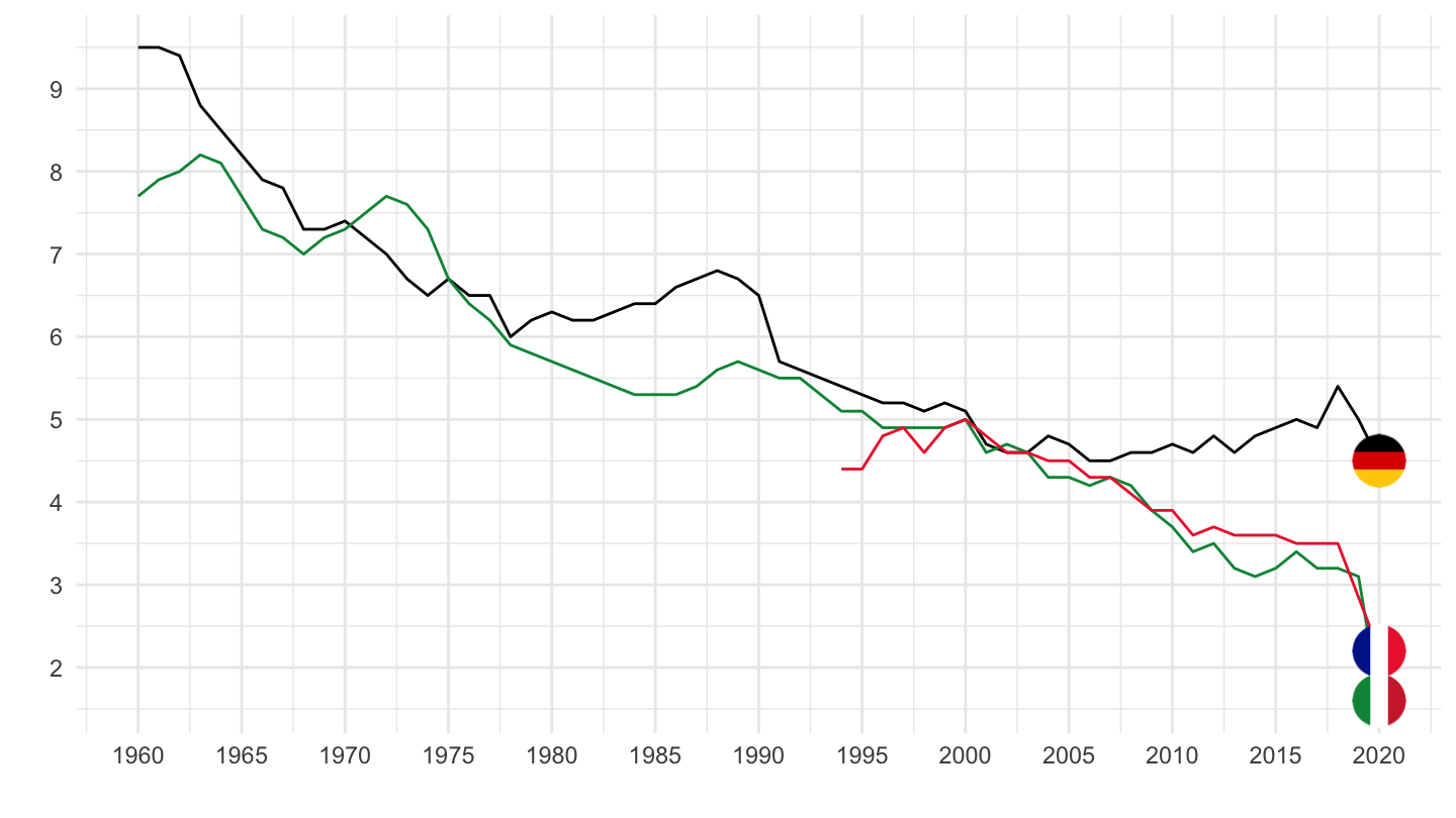
Crude divorce rate (divorces per 1000 people) - FAM4B
Table
Code
FAMILY %>%
  filter(IND == "FAM4B") %>%
  left_join(FAMILY_var$COU, by = "COU") %>%
  group_by(COU, Cou) %>%
  summarise(Nobs = n(),
            obsTime = last(obsTime),
            obsValue = last(obsValue)) %>%
  mutate(Flag = gsub(" ", "-", str_to_lower(Cou)),
         Flag = paste0('<img src="../../icon/flag/vsmall/', Flag, '.png" alt="Flag">')) %>%
  select(Flag, everything()) %>%
  {if (is_html_output()) datatable(., filter = 'top', rownames = F, escape = F) else .}
France, Italy, Germany
Code
FAMILY %>%
  filter(IND == "FAM4B",
         COU %in% c("FRA", "DEU", "ITA")) %>%
  year_to_date() %>%
  left_join(FAMILY_var$COU, by = "COU") %>%
  rename(Location = Cou) %>%
  left_join(colors, by = c("Location" = "country")) %>%
  ggplot(.) + theme_minimal() + scale_color_identity() +
  geom_line(aes(x = date, y = obsValue, color = color)) +
  xlab("") + ylab("") + add_3flags +
  scale_x_date(breaks = seq(1940, 2050, 5) %>% paste0("-01-01") %>% as.Date,
               labels = date_format("%Y")) +
  scale_y_continuous(breaks = seq(0, 10, .2))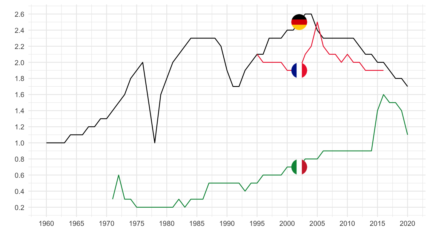
Infant mortality rate - FAM16A
Table
Code
FAMILY %>%
  filter(IND == "FAM16A") %>%
  left_join(FAMILY_var$COU, by = "COU") %>%
  group_by(COU, Cou) %>%
  summarise(Nobs = n(),
            obsTime = last(obsTime),
            obsValue = last(obsValue)) %>%
  arrange(obsValue) %>%
  mutate(Flag = gsub(" ", "-", str_to_lower(Cou)),
         Flag = paste0('<img src="../../icon/flag/vsmall/', Flag, '.png" alt="Flag">')) %>%
  select(Flag, everything()) %>%
  {if (is_html_output()) datatable(., filter = 'top', rownames = F, escape = F) else .}
France
All
Code
FAMILY %>%
  filter(IND == "FAM16A",
         COU %in% c("FRA")) %>%
  add_row(obsTime = "2020", obsValue = 3.6 ) %>%
  add_row(obsTime = "2021", obsValue = 3.7 ) %>%
  add_row(obsTime = "2022", obsValue = 3.9 ) %>%
  add_row(obsTime = "2023", obsValue = 4 ) %>%
  year_to_date() %>%
  left_join(FAMILY_var$COU, by = "COU") %>%
  rename(Location = Cou) %>%
  left_join(colors, by = c("Location" = "country")) %>%
  ggplot(.) + theme_minimal() + scale_color_identity() +
  geom_line(aes(x = date, y = obsValue)) +
  xlab("") + ylab("") + add_3flags +
  scale_x_date(breaks = seq(1940, 2050, 5) %>% paste0("-01-01") %>% as.Date,
               labels = date_format("%Y")) +
  scale_y_continuous(breaks = seq(0, 100, 5),
                     labels = dollar_format(a = .1, pre = "", su = "‰"))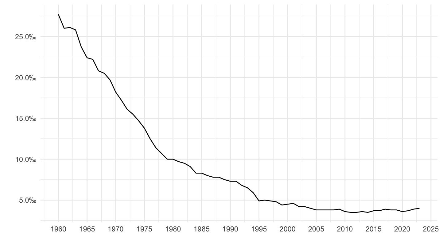
1980-
Code
FAMILY %>%
  filter(IND == "FAM16A",
         COU %in% c("FRA")) %>%
  add_row(obsTime = "2020", obsValue = 3.6 ) %>%
  add_row(obsTime = "2021", obsValue = 3.7 ) %>%
  add_row(obsTime = "2022", obsValue = 3.9 ) %>%
  add_row(obsTime = "2023", obsValue = 4 ) %>%
  year_to_date() %>%
  filter(date >= as.Date("1991-01-01")) %>%
  left_join(FAMILY_var$COU, by = "COU") %>%
  rename(Location = Cou) %>%
  left_join(colors, by = c("Location" = "country")) %>%
  ggplot(.) + theme_minimal() + scale_color_identity() +
  geom_line(aes(x = date, y = obsValue)) +
  ylab("Taux de mortalité infantile (pour mille)") + xlab("") + add_3flags +
  scale_x_date(breaks = seq(1991, 2050, 2) %>% paste0("-01-01") %>% as.Date,
               labels = date_format("%Y")) +
  scale_y_continuous(breaks = seq(0, 100, 1),
                     labels = dollar_format(a = .1, pre = "", su = "‰")) +
  theme(legend.position = c(0.2, 0.7),
        legend.title = element_blank(),
        axis.text.x = element_text(angle = 45, vjust = 1, hjust = 1))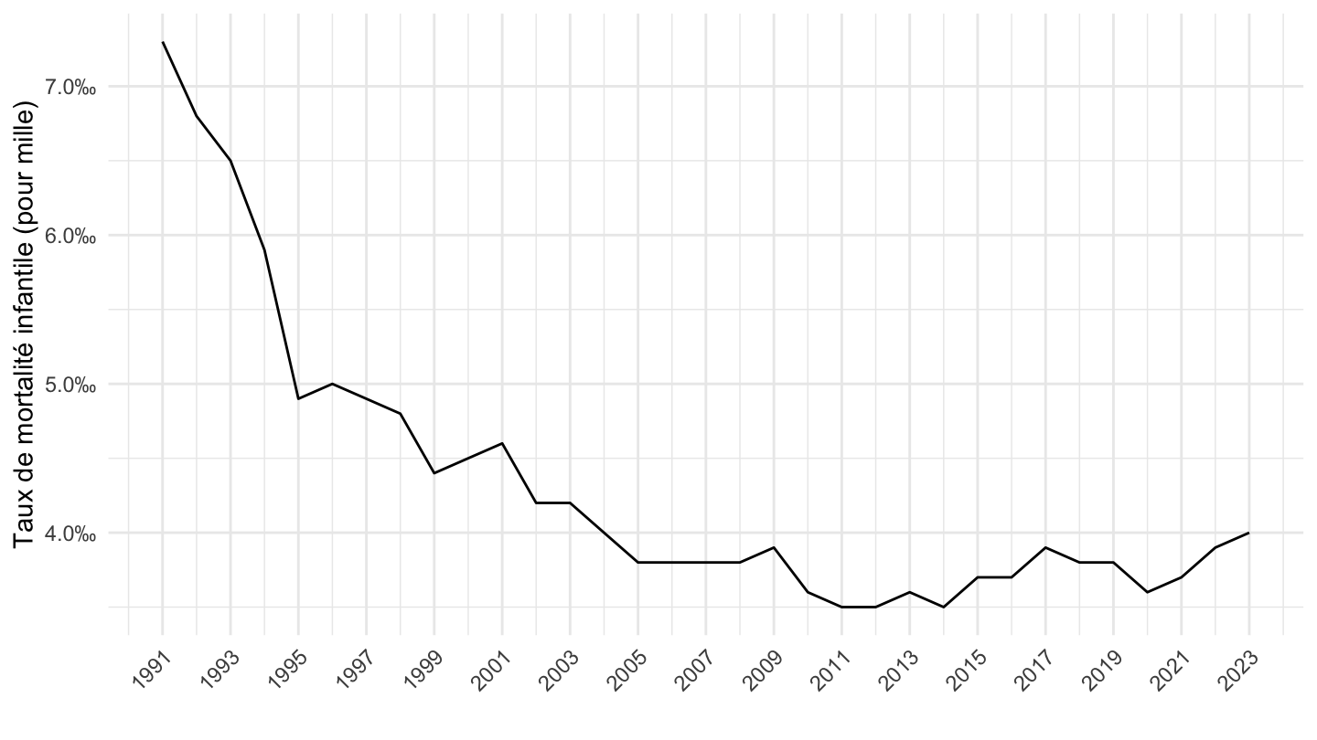
France, Italy, Germany, Spain, Portugal
All
Code
FAMILY %>%
  filter(IND == "FAM16A",
         COU %in% c("FRA", "DEU", "ITA", "ESP", "PRT")) %>%
  year_to_date() %>%
  left_join(FAMILY_var$COU, by = "COU") %>%
  rename(Location = Cou) %>%
  left_join(colors, by = c("Location" = "country")) %>%
  ggplot(.) + theme_minimal() + scale_color_identity() +
  geom_line(aes(x = date, y = obsValue, color = color)) +
  xlab("") + ylab("") + add_3flags +
  scale_x_date(breaks = seq(1940, 2050, 5) %>% paste0("-01-01") %>% as.Date,
               labels = date_format("%Y")) +
  scale_y_continuous(breaks = seq(0, 100, 5))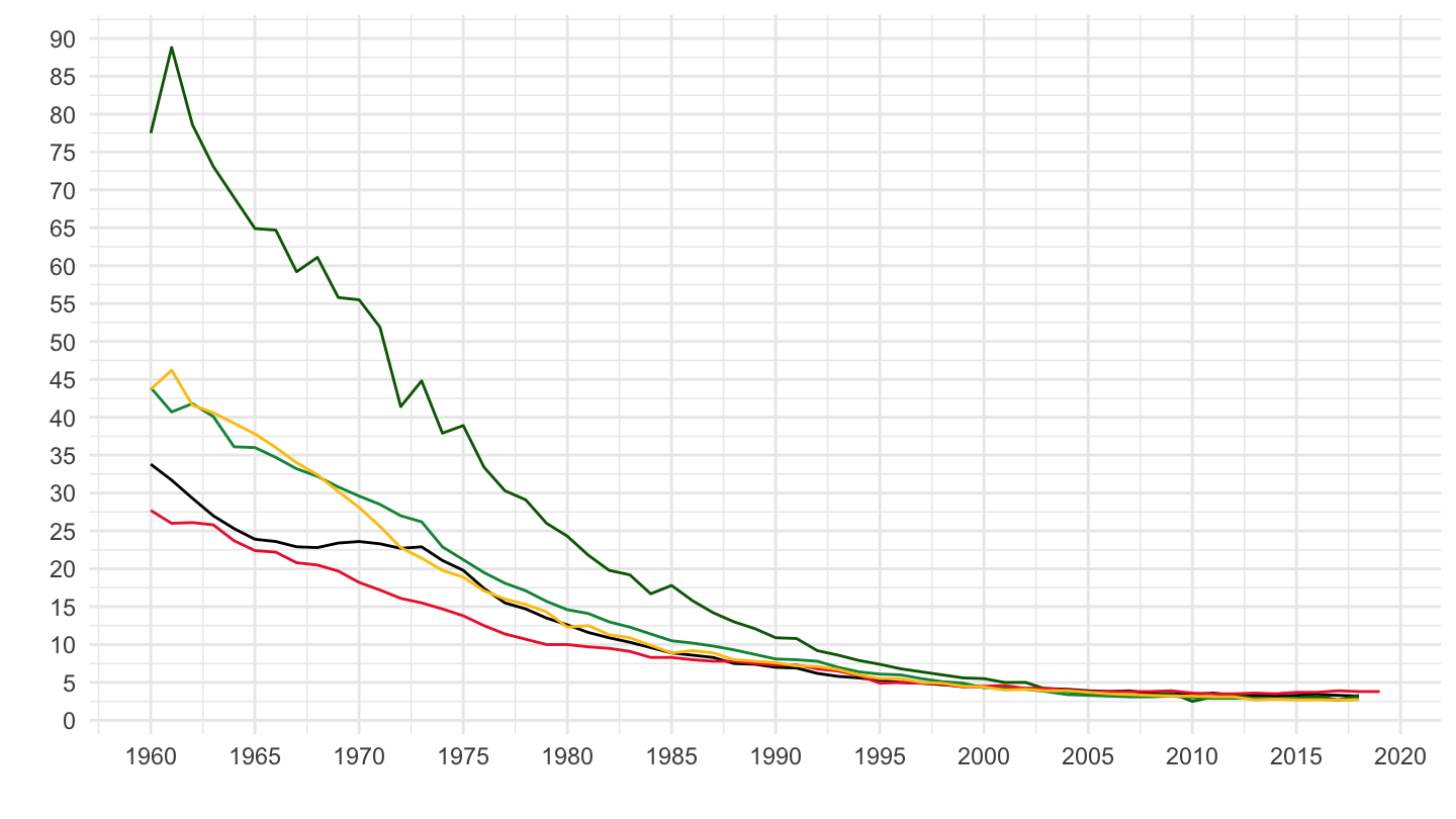
Log
Code
FAMILY %>%
  filter(IND == "FAM16A",
         COU %in% c("FRA", "DEU", "ITA", "ESP")) %>%
  # Source: 2020,2021 = Eurostat, demo_minfind; 2022-2023: INSEE
  add_row(COU = "DEU", obsTime = "2020", obsValue = 3.1 ) %>%
  add_row(COU = "DEU", obsTime = "2021", obsValue = 3 ) %>%
  add_row(COU = "ITA", obsTime = "2020", obsValue = 2.4 ) %>%
  add_row(COU = "ITA", obsTime = "2021", obsValue = 2.3 ) %>%
  add_row(COU = "ESP", obsTime = "2020", obsValue = 2.6 ) %>%
  add_row(COU = "ESP", obsTime = "2021", obsValue = 2.5 ) %>%
  add_row(COU = "FRA", obsTime = "2020", obsValue = 3.6 ) %>%
  add_row(COU = "FRA", obsTime = "2021", obsValue = 3.7 ) %>%
  add_row(COU = "FRA", obsTime = "2022", obsValue = 3.9 ) %>%
  add_row(COU = "FRA", obsTime = "2023", obsValue = 4 ) %>%
  year_to_date() %>%
  left_join(FAMILY_var$COU, by = "COU") %>%
  rename(Location = Cou) %>%
  left_join(colors, by = c("Location" = "country")) %>%
  mutate(color = ifelse(COU == "PRT", color2, color)) %>%
  arrange(desc(date)) %>%
  ggplot(.) + theme_minimal() + scale_color_identity() +
  geom_line(aes(x = date, y = obsValue, color = color)) +
  xlab("") + ylab("Taux de mortalité infantile (‰)") + add_4flags +
  scale_x_date(breaks = seq(1940, 2050, 10) %>% paste0("-01-01") %>% as.Date,
               labels = date_format("%Y")) +
  scale_y_log10(breaks = c(seq(0, 100, 10), 6, 8, 15, 25, seq(1, 5, 1)),
                     labels = dollar_format(a = .1, pre = "", su = "‰"))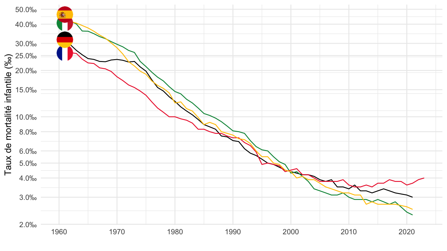
2000-
Code
FAMILY %>%
  filter(IND == "FAM16A",
         COU %in% c("FRA", "DEU", "ITA")) %>%
  year_to_date() %>%
  filter(date >= as.Date("2000-01-01")) %>%
  left_join(FAMILY_var$COU, by = "COU") %>%
  rename(Location = Cou) %>%
  left_join(colors, by = c("Location" = "country")) %>%
  ggplot(.) + theme_minimal() + scale_color_identity() +
  geom_line(aes(x = date, y = obsValue, color = color)) +
  xlab("") + ylab("Taux de mortalité infantile (‰)") + add_3flags +
  scale_x_date(breaks = seq(1940, 2050, 2) %>% paste0("-01-01") %>% as.Date,
               labels = date_format("%Y")) +
  scale_y_continuous(breaks = seq(0, 100, .2),
                     labels = dollar_format(a = .1, pre = "", su = "‰"))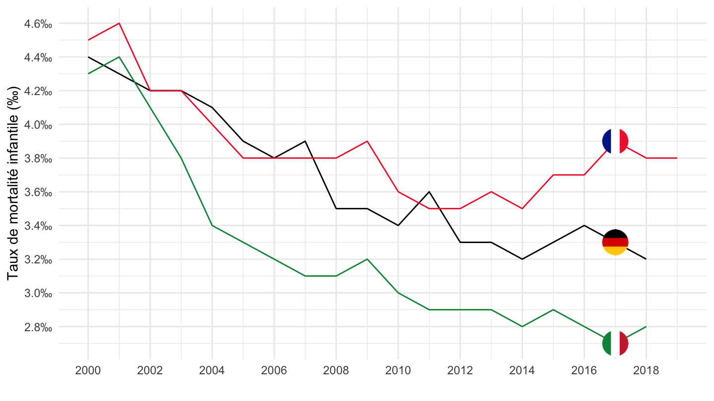
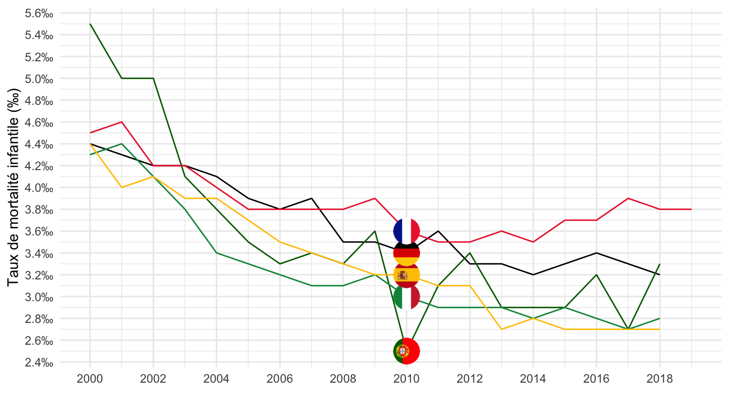
2000-
Code
FAMILY %>%
  filter(IND == "FAM16A",
         COU %in% c("FRA", "DEU", "ITA", "PRT", "ESP")) %>%
  year_to_date() %>%
  filter(date >= as.Date("2000-01-01")) %>%
  left_join(FAMILY_var$COU, by = "COU") %>%
  rename(Location = Cou) %>%
  left_join(colors, by = c("Location" = "country")) %>%
  ggplot(.) + theme_minimal() + scale_color_identity() +
  geom_line(aes(x = date, y = obsValue, color = color)) +
  xlab("") + ylab("Taux de mortalité infantile (‰)") + add_5flags +
  scale_x_date(breaks = seq(1940, 2050, 2) %>% paste0("-01-01") %>% as.Date,
               labels = date_format("%Y")) +
  scale_y_continuous(breaks = seq(0, 100, .2),
                     labels = dollar_format(a = .1, pre = "", su = "‰"))