Table 1.1.5. Gross Domestic Product (A) (Q)
Data - BEA
Info
Data on US macro
LAST_COMPILE
| LAST_COMPILE |
|---|
| 2025-04-09 |
Last
| TimePeriod | Nobs |
|---|---|
| 2024Q4 | 26 |
Layout
- NIPA Website. html
LineNumber, LineDescription
Code
T10105_A %>%
  group_by(LineNumber, LineDescription, SeriesCode) %>%
  summarise(Nobs = n()) %>%
print_table_conditional()| LineNumber | LineDescription | SeriesCode | Nobs |
|---|---|---|---|
| 1 | Gross domestic product | A191RC | 96 |
| 2 | Personal consumption expenditures | DPCERC | 96 |
| 3 | Goods | DGDSRC | 96 |
| 4 | Durable goods | DDURRC | 96 |
| 5 | Nondurable goods | DNDGRC | 96 |
| 6 | Services | DSERRC | 96 |
| 7 | Gross private domestic investment | A006RC | 96 |
| 8 | Fixed investment | A007RC | 96 |
| 9 | Nonresidential | A008RC | 96 |
| 10 | Structures | B009RC | 96 |
| 11 | Equipment | Y033RC | 96 |
| 12 | Intellectual property products | Y001RC | 96 |
| 13 | Residential | A011RC | 96 |
| 14 | Change in private inventories | A014RC | 96 |
| 15 | Net exports of goods and services | A019RC | 96 |
| 16 | Exports | B020RC | 96 |
| 17 | Goods | A253RC | 96 |
| 18 | Services | A646RC | 96 |
| 19 | Imports | B021RC | 96 |
| 20 | Goods | A255RC | 96 |
| 21 | Services | B656RC | 96 |
| 22 | Government consumption expenditures and gross investment | A822RC | 96 |
| 23 | Federal | A823RC | 96 |
| 24 | National defense | A824RC | 96 |
| 25 | Nondefense | A825RC | 96 |
| 26 | State and local | A829RC | 96 |
Imports and Exports
Graph, Annual
Code
T10105_A %>%
  year_to_date %>%
  filter(LineNumber %in% c(1, 16, 19)) %>%
  group_by(date) %>%
  transmute(date,
            `Exports` = DataValue[LineNumber == 16]/DataValue[LineNumber == 1],
            `Imports` = DataValue[LineNumber == 19]/DataValue[LineNumber == 1]) %>%
  gather(variable, value, -date) %>%
  ggplot(.) + theme_minimal() + xlab("") +  ylab("Exports, Imports (% of GDP)") +
  geom_line(aes(x = date, y = value, color = variable, linetype = variable)) +
  scale_x_date(breaks = seq(1920, 2100, 5) %>% paste0("-01-01") %>% as.Date,
               labels = date_format("%Y")) +
  scale_color_manual(values = viridis(3)[1:2]) +
  theme(legend.title = element_blank(),
        legend.position = c(0.2, 0.9)) +
  scale_y_continuous(breaks = seq(-0.06, 0.4, 0.02),
                     labels = scales::percent_format(accuracy = 1))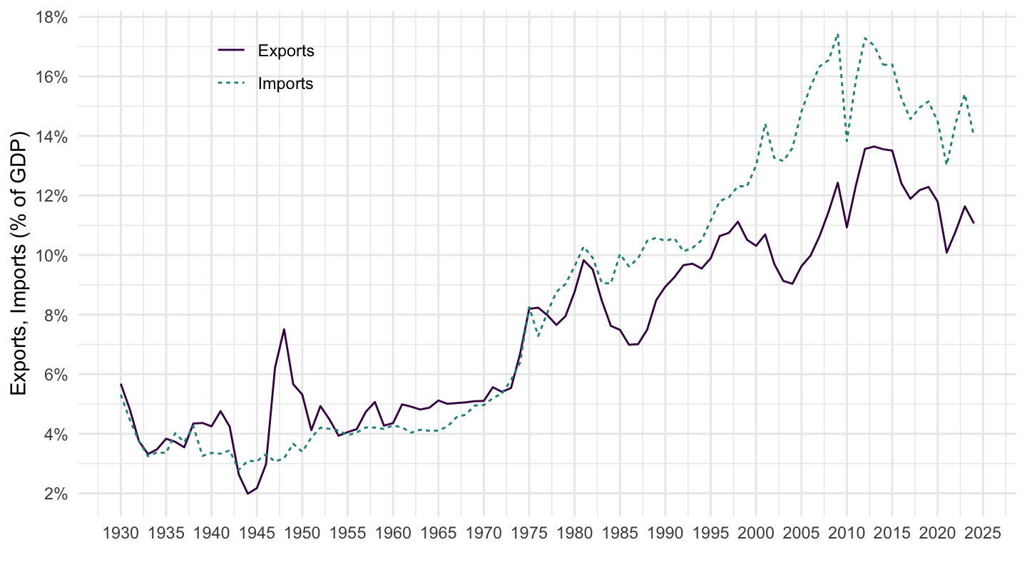
Goods, Services
Code
T10105_A %>%
  year_to_date %>%
  filter(LineNumber %in% c(1, 17, 18, 20, 21)) %>%
  group_by(date) %>%
  transmute(date,
            `Exports - Goods` = DataValue[LineNumber == 17]/DataValue[LineNumber == 1],
            `Exports - Services` = DataValue[LineNumber == 18]/DataValue[LineNumber == 1],
            `Imports - Goods` = DataValue[LineNumber == 20]/DataValue[LineNumber == 1],
            `Imports - Services` = DataValue[LineNumber == 21]/DataValue[LineNumber == 1]) %>%
  gather(variable, value, -date) %>%
  ggplot(.) + theme_minimal() + xlab("") +  ylab("Exports, Imports (% of GDP)") +
  geom_line(aes(x = date, y = value, color = variable, linetype = variable)) +
  scale_x_date(breaks = seq(1920, 2100, 5) %>% paste0("-01-01") %>% as.Date,
               labels = date_format("%Y")) +
  scale_color_manual(values = c(viridis(3)[1], viridis(3)[2], viridis(3)[1], viridis(3)[2])) +
  scale_linetype_manual(values = c("dashed", "dashed", "solid",  "solid")) +
  theme(legend.title = element_blank(),
        legend.position = c(0.2, 0.9)) +
  scale_y_continuous(breaks = seq(-0.06, 0.4, 0.02),
                     labels = scales::percent_format(accuracy = 1))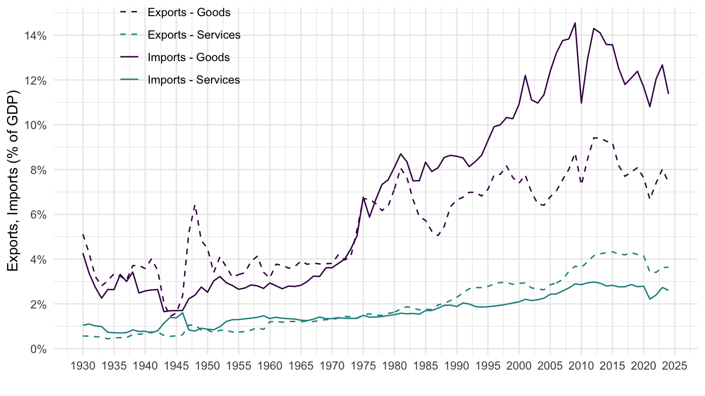
Goods, Services with NBER Recessions
Code
T10105_A %>%
  year_to_date %>%
  filter(LineNumber %in% c(1, 17, 18, 20, 21)) %>%
  group_by(date) %>%
  transmute(date,
            `Exports - Goods` = DataValue[LineNumber == 17]/DataValue[LineNumber == 1],
            `Exports - Services` = DataValue[LineNumber == 18]/DataValue[LineNumber == 1],
            `Imports - Goods` = DataValue[LineNumber == 20]/DataValue[LineNumber == 1],
            `Imports - Services` = DataValue[LineNumber == 21]/DataValue[LineNumber == 1]) %>%
  gather(variable, value, -date) %>%
  ggplot(.) + theme_minimal() + xlab("") +  ylab("Exports, Imports (% of GDP)") +
  geom_line(aes(x = date, y = value, color = variable, linetype = variable)) +
  scale_x_date(breaks = seq(1920, 2100, 5) %>% paste0("-01-01") %>% as.Date,
               labels = date_format("%Y")) +
  scale_color_manual(values = c(viridis(3)[1], viridis(3)[2], viridis(3)[1], viridis(3)[2])) +
  scale_linetype_manual(values = c("dashed", "dashed", "solid",  "solid")) +
  geom_rect(data = nber_recessions %>%
              filter(Peak > as.Date("1928-01-01")),
            aes(xmin = Peak, xmax = Trough, ymin = -Inf, ymax = +Inf),
            fill = 'grey', alpha = 0.5) +
  theme(legend.title = element_blank(),
        legend.position = c(0.2, 0.9)) +
  scale_y_continuous(breaks = seq(-0.06, 0.4, 0.02),
                     labels = scales::percent_format(accuracy = 1))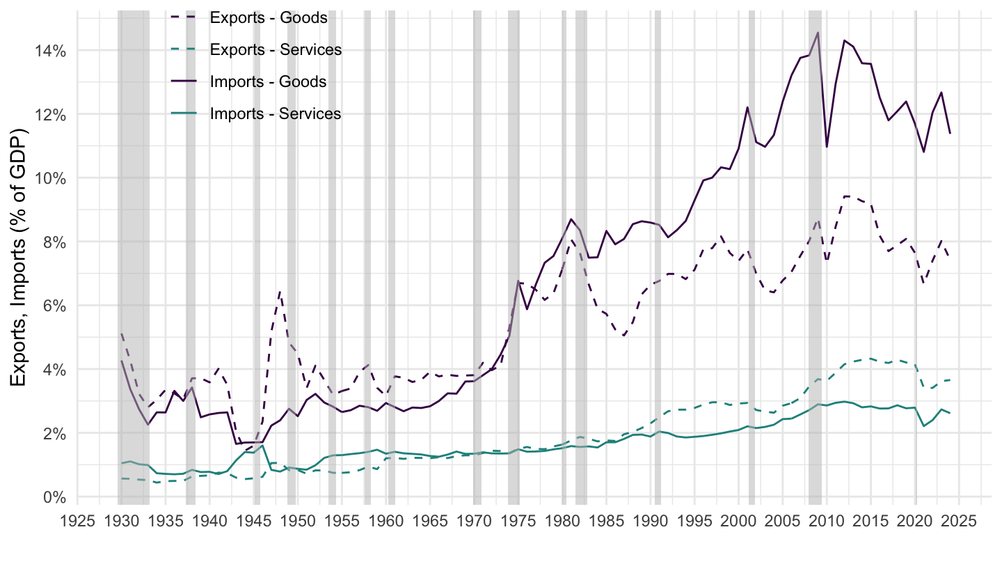
Net Exports, Goods and Services
Graph with Presidents
Code
US_presidents_extract <- US_presidents %>%
  filter(start >= as.Date("1945-01-01"))
T10105_Q %>%
  quarter_to_date %>%
  filter(LineNumber %in% c(1, 16:21)) %>%
  select(date, DataValue, LineNumber) %>%
  spread(LineNumber, DataValue) %>%
  transmute(date,
            `Net exports of goods and services` = (`16`-`19`)/`1`,
         `Net exports of goods` = (`17`-`20`)/`1`,
         `Net exports of services` = (`18`-`21`)/`1`) %>%
  gather(variable, value, -date) %>%
  mutate(variable = factor(variable, levels = c("Net exports of services",
                                                "Net exports of goods and services",
                                                "Net exports of goods"))) %>%
  ggplot(.) + theme_minimal() + xlab("") +  ylab("Net Exports (% of GDP)") +
  geom_line(aes(x = date, y = value, color = variable)) +
  theme(legend.title = element_blank(),
        legend.position = c(0.25, 0.35),
        axis.text.x = element_text(angle = 45, vjust = 1, hjust = 1)) +
  scale_x_date(breaks = as.Date(US_presidents_extract$start),
               labels = date_format("%Y")) +
  geom_vline(aes(xintercept = as.numeric(start)),
             data = US_presidents,
             colour = "grey50", alpha = 0.5) +
  geom_text(aes(x = start, y = new, label = name),
            data = US_presidents_extract %>% mutate(new = -0.08 + 0.005 * (1:n() %% 2)),
            size = 2.5, vjust = 0, hjust = 0, nudge_x = 50) +
  geom_rect(aes(xmin = start, xmax = end, fill = party),
         ymin = -Inf, ymax = Inf, alpha = 0.1, data = US_presidents_extract) +
  scale_fill_manual(values = c("white", "grey")) +
  guides(color = guide_legend("party"), fill = FALSE) +
  scale_y_continuous(breaks = seq(-0.1, 0.05, 0.01),
                     labels = scales::percent_format(accuracy = 1)) +
  geom_hline(yintercept = 0, linetype = "dashed",  color = viridis(3)[2])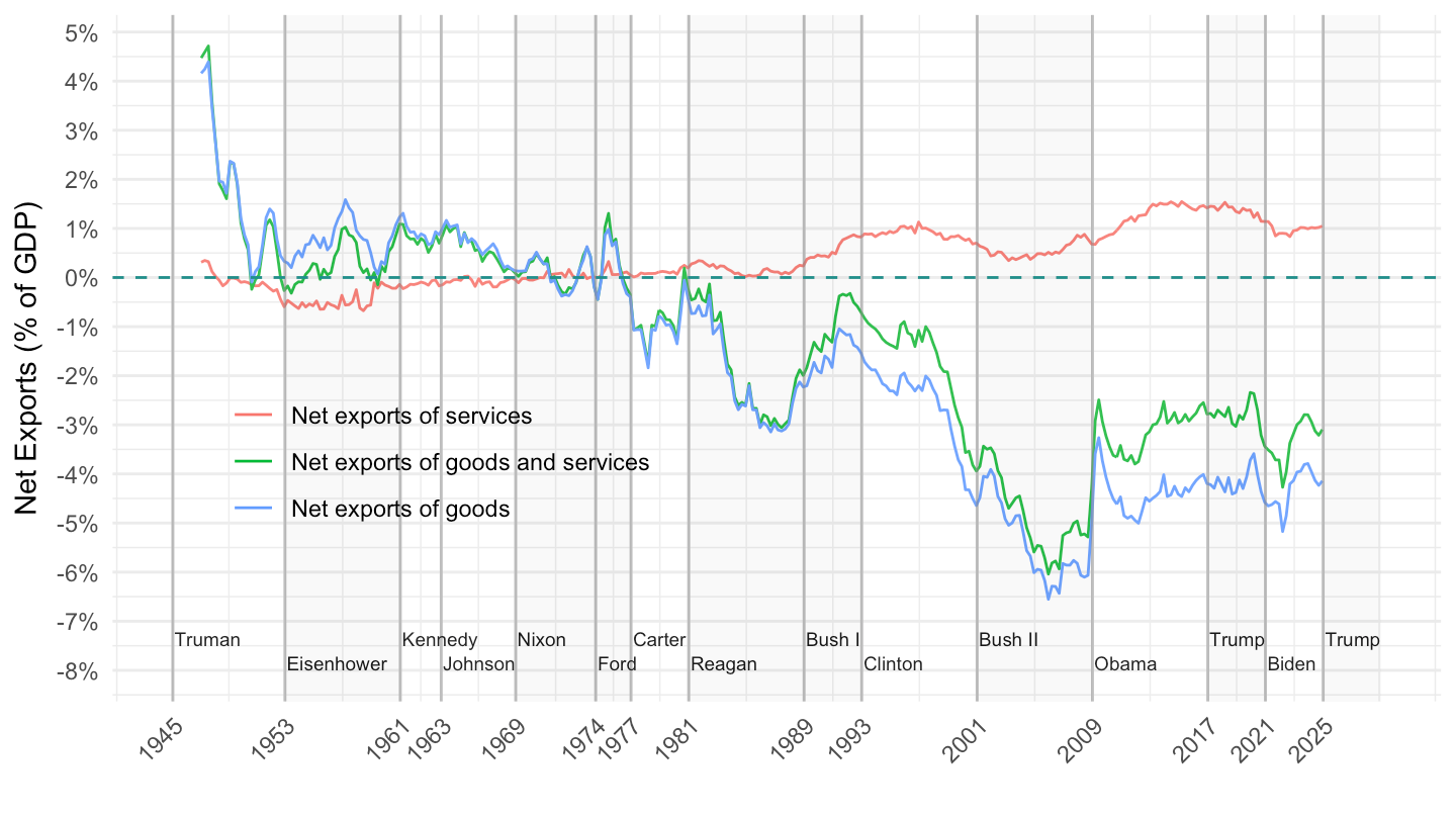
Net Exports
Quarterly
Code
T10105_Q %>%
  quarter_to_date %>%
  filter(LineNumber %in% c(1, 15)) %>%
  group_by(date) %>%
  mutate(net_exports_gdp = DataValue[LineNumber == 15]/DataValue[LineNumber == 1]) %>%
  ggplot(.) + theme_minimal() + xlab("") +  ylab("Net Exports (% of GDP)") +
  geom_line(aes(x = date, y = net_exports_gdp)) +
  scale_x_date(breaks = seq(1920, 2100, 5) %>% paste0("-01-01") %>% as.Date,
               labels = date_format("%Y")) +
  theme(legend.title = element_blank(),
        legend.position = c(0.4, 0.8)) +
  scale_y_continuous(breaks = seq(-0.06, 0.05, 0.01),
                     labels = scales::percent_format(accuracy = 1)) +
  geom_hline(yintercept = 0, linetype = "dashed",  color = viridis(3)[2])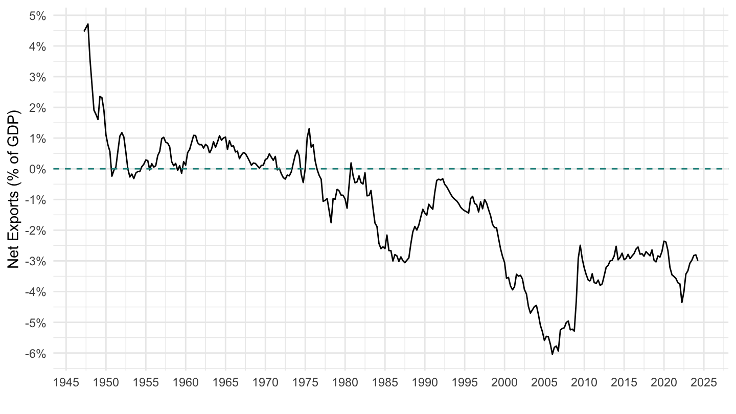
Annual
Code
T10105_A %>%
  year_to_date %>%
  filter(LineNumber %in% c(1, 15)) %>%
  group_by(date) %>%
  mutate(net_exports_gdp = DataValue[LineNumber == 15]/DataValue[LineNumber == 1]) %>%
  ggplot(.) + theme_minimal() + xlab("") +  ylab("Net Exports (% of GDP)") +
  geom_line(aes(x = date, y = net_exports_gdp)) +
  scale_x_date(breaks = seq(1920, 2100, 5) %>% paste0("-01-01") %>% as.Date,
               labels = date_format("%Y")) +
  theme(legend.title = element_blank(),
        legend.position = c(0.4, 0.8)) +
  scale_y_continuous(breaks = seq(-0.06, 0.05, 0.01),
                     labels = scales::percent_format(accuracy = 1)) +
  geom_hline(yintercept = 0, linetype = "dashed",  color = viridis(3)[2])
Graph with Presidents
Code
US_presidents_extract <- US_presidents %>%
  filter(start >= as.Date("1945-01-01"))
T10105_Q %>%
  quarter_to_date %>%
  filter(LineNumber %in% c(1, 15)) %>%
  group_by(date) %>%
  mutate(net_exports_gdp = DataValue[LineNumber == 15]/DataValue[LineNumber == 1]) %>%
  ggplot(.) + theme_minimal() + xlab("") +  ylab("Net Exports (% of GDP)") +
  geom_line(aes(x = date, y = net_exports_gdp)) +
  theme(legend.title = element_blank(),
        legend.position = c(0.4, 0.8)) +
  scale_x_date(breaks = as.Date(US_presidents_extract$start),
               labels = date_format("%Y")) +
  geom_vline(aes(xintercept = as.numeric(start)),
             data = US_presidents,
             colour = "grey50", alpha = 0.5) +
  geom_text(aes(x = start, y = new, label = name),
            data = US_presidents_extract %>% mutate(new = -0.08 + 0.005 * (1:n() %% 2)),
            size = 2.5, vjust = 0, hjust = 0, nudge_x = 50) +
  geom_rect(aes(xmin = start, xmax = end, fill = party),
         ymin = -Inf, ymax = Inf, alpha = 0.1, data = US_presidents_extract) +
  scale_fill_manual(values = c("white", "grey")) +
  guides(color = guide_legend("party"), fill = FALSE) +
  scale_y_continuous(breaks = seq(-0.06, 0.05, 0.01),
                     labels = scales::percent_format(accuracy = 1)) +
  geom_hline(yintercept = 0, linetype = "dashed",  color = viridis(3)[2])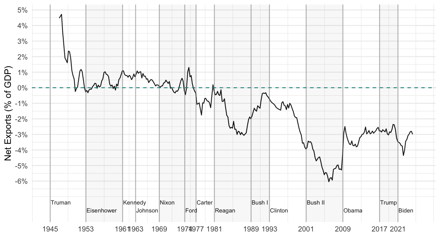
Data
Code
T10105_Q %>%
  quarter_to_date %>%
  filter(SeriesCode %in% c("A191RC", "A019RC"),
         date >= as.Date("2016-12-01")) %>%
  select(SeriesCode, date, DataValue) %>%
  spread(SeriesCode, DataValue) %>%
  {if (is_html_output()) datatable(., filter = 'top', rownames = F) else .}
Data - Plots
Code
T10105_Q %>%
  quarter_to_date %>%
  filter(SeriesCode %in% c("A191RC", "A019RC"),
         date >= as.Date("2017-01-01")) %>%
  select(SeriesCode, date, DataValue) %>%
  spread(SeriesCode, DataValue) %>%
  ggplot() + geom_line(aes(x = date, y = A019RC/1000)) +
  theme_minimal() +
  scale_x_date(breaks = as.Date(paste0(seq(1960, 2024, 1), "-01-01")),
               labels = date_format("%Y")) +
  theme(legend.position = c(0.2, 0.85),
        legend.title = element_blank()) +
  xlab("") + ylab("") +
  scale_y_continuous(breaks = seq(-2000, 2000, 100),
                labels = dollar_format(suffix = " Bn", accuracy = 1))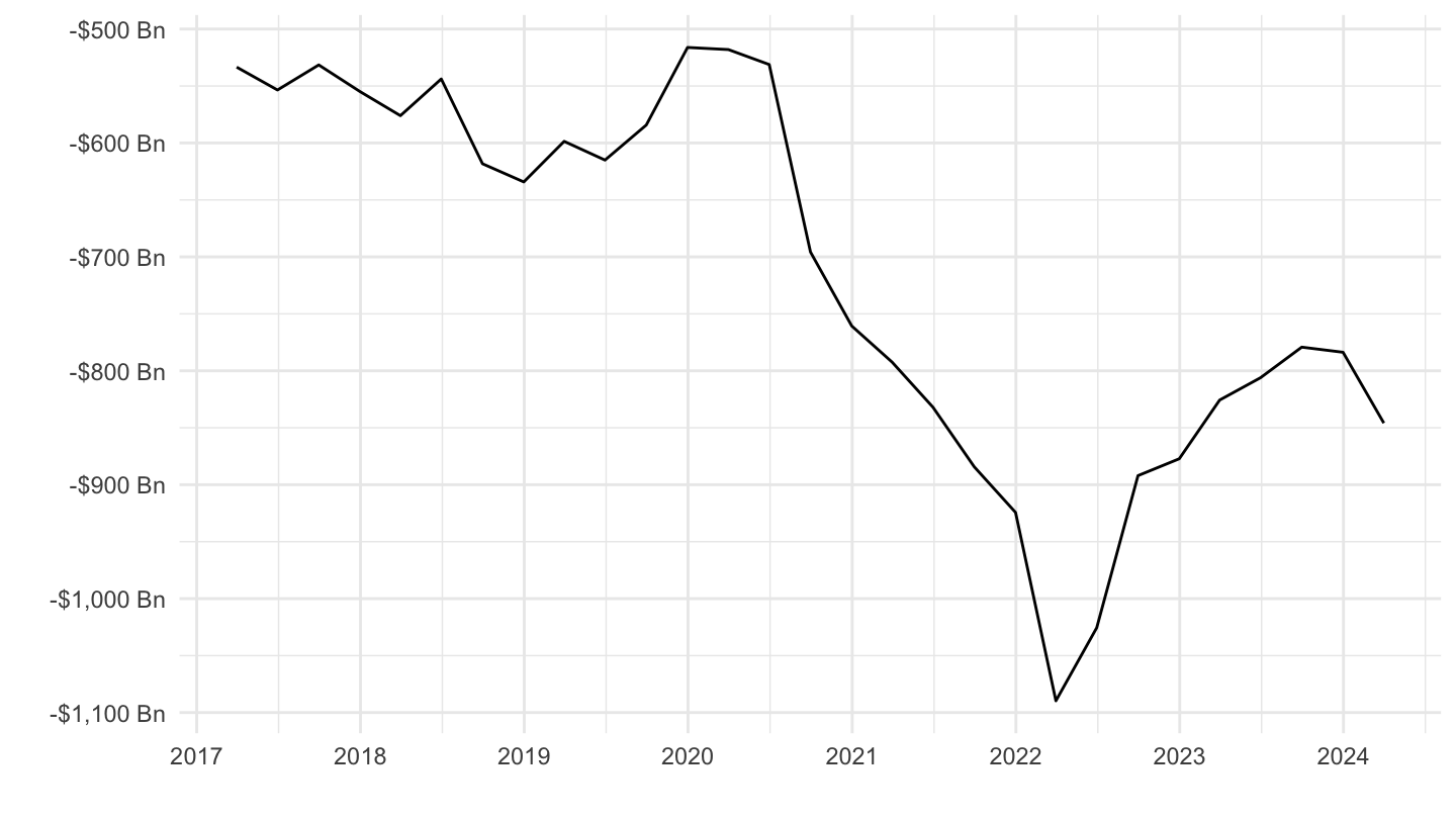
1938, 1958, 1978, 1998, 2018 Table
Percent
Code
T10105_A %>%
  year_to_date %>%
  mutate(year = year(date)) %>%
  filter(year %in% c(1929, 1949, 1969, 1989, 2009, 2019)) %>%
  group_by(year) %>%
  mutate(value = round(100*DataValue/DataValue[1], 1)) %>%
  ungroup %>%
  select(2, 3, 6, 7) %>%
  spread(year, value) %>%
  mutate_at(vars(-1, -2), funs(ifelse(is.na(.), "", paste0(., " %")))) %>%
  select(-LineNumber) %>%
  setNames(c("", names(.)[2:7])) %>%
  knitr::kable(booktabs = TRUE,
               linesep = "") %>%
  kable_styling(bootstrap_options = c("striped", "hover", "condensed"),
                latex_options = c("striped", "hold_position")) %>%
  add_indent(c(2:26)) %>%
  add_indent(c(3:6, 8:14, 16:21, 23:26)) %>%
  add_indent(c(4:5, 9:13, 17:18, 20:21, 24:25)) %>%
add_indent(c(10:12))| 1929 | 1949 | 1969 | 1989 | 2009 | 2019 | |
|---|---|---|---|---|---|---|
| Gross domestic product | 100 % | 100 % | 100 % | 100 % | 100 % | 100 % |
| Personal consumption expenditures | 74 % | 65.4 % | 59.3 % | 63.4 % | 68.3 % | 67 % |
| Goods | 41.9 % | 39.7 % | 29.9 % | 25.2 % | 22 % | 21 % |
| Durable goods | 9.4 % | 9.8 % | 8.9 % | 8.8 % | 7 % | 7.1 % |
| Nondurable goods | 32.5 % | 29.9 % | 21 % | 16.5 % | 15 % | 14 % |
| Services | 32.1 % | 25.8 % | 29.4 % | 38.2 % | 46.4 % | 46 % |
| Gross private domestic investment | 16.4 % | 14.3 % | 17.1 % | 17.7 % | 13.3 % | 18.1 % |
| Fixed investment | 14.9 % | 15.3 % | 16.2 % | 17.2 % | 14.4 % | 17.7 % |
| Nonresidential | 11.1 % | 9.9 % | 11.8 % | 12.7 % | 11.7 % | 13.9 % |
| Structures | 5.3 % | 3.4 % | 3.7 % | 3.4 % | 3.1 % | 3.1 % |
| Equipment | 5.3 % | 5.8 % | 6.4 % | 6.6 % | 4.6 % | 5.8 % |
| Intellectual property products | 0.6 % | 0.7 % | 1.7 % | 2.7 % | 3.9 % | 5 % |
| Residential | 3.9 % | 5.4 % | 4.4 % | 4.5 % | 2.7 % | 3.8 % |
| Change in private inventories | 1.5 % | -1 % | 0.9 % | 0.5 % | -1 % | 0.3 % |
| Net exports of goods and services | 0.4 % | 1.9 % | 0.1 % | -1.5 % | -2.9 % | -2.7 % |
| Exports | 5.7 % | 5.3 % | 5.1 % | 8.9 % | 10.9 % | 11.8 % |
| Goods | 5.1 % | 4.5 % | 3.8 % | 6.6 % | 7.3 % | 7.6 % |
| Services | 0.6 % | 0.8 % | 1.3 % | 2.3 % | 3.6 % | 4.2 % |
| Imports | 5.3 % | 3.4 % | 5 % | 10.5 % | 13.8 % | 14.5 % |
| Goods | 4.3 % | 2.5 % | 3.6 % | 8.6 % | 11 % | 11.7 % |
| Services | 1 % | 0.9 % | 1.3 % | 1.9 % | 2.9 % | 2.8 % |
| Government consumption expenditures and gross investment | 9.2 % | 18.3 % | 23.5 % | 20.4 % | 21.2 % | 17.6 % |
| Federal | 1.8 % | 11.2 % | 12.9 % | 9.5 % | 8.4 % | 6.6 % |
| National defense | 1 % | 8.2 % | 10 % | 6.9 % | 5.4 % | 3.9 % |
| Nondefense | 0.8 % | 3 % | 2.9 % | 2.5 % | 3 % | 2.6 % |
| State and local | 7.4 % | 7.1 % | 10.6 % | 11 % | 12.8 % | 11 % |
Percent - pdf
Code
include_graphics2("https://fgeerolf.com/bib/bea/T10105_ex.png")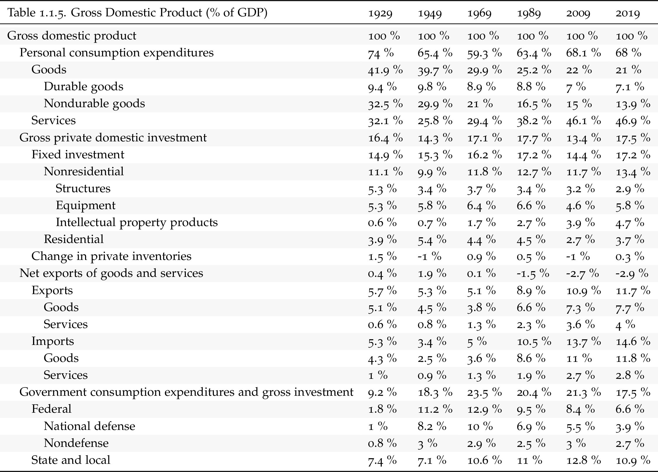
Billions
Code
T10105_A %>%
  year_to_date %>%
  mutate(year = year(date)) %>%
  filter(year %in% c(1929, 1949, 1969, 1989, 2009, 2019)) %>%
  group_by(year) %>%
  mutate(value = round(DataValue/1000)) %>%
  ungroup %>%
  select(2, 3, 6, 7) %>%
  spread(year, value) %>%
  mutate_at(vars(-1, -2), funs(ifelse(is.na(.), "", paste0("$ ",., " Bn")))) %>%
  select(-LineNumber) %>%
  setNames(c("", names(.)[2:7])) %>%
  knitr::kable(booktabs = TRUE,
               linesep = "") %>%
  kable_styling(bootstrap_options = c("striped", "hover", "condensed"),
                latex_options = c("striped", "hold_position")) %>%
  add_indent(c(2:26)) %>%
  add_indent(c(3:6, 8:14, 16:21, 23:26)) %>%
  add_indent(c(4:5, 9:13, 17:18, 20:21, 24:25)) %>%
add_indent(c(10:12))| 1929 | 1949 | 1969 | 1989 | 2009 | 2019 | |
|---|---|---|---|---|---|---|
| Gross domestic product | $ 105 Bn | $ 272 Bn | $ 1018 Bn | $ 5642 Bn | $ 14478 Bn | $ 21540 Bn |
| Personal consumption expenditures | $ 77 Bn | $ 178 Bn | $ 604 Bn | $ 3577 Bn | $ 9891 Bn | $ 14438 Bn |
| Goods | $ 44 Bn | $ 108 Bn | $ 305 Bn | $ 1424 Bn | $ 3180 Bn | $ 4533 Bn |
| Durable goods | $ 10 Bn | $ 27 Bn | $ 90 Bn | $ 494 Bn | $ 1012 Bn | $ 1524 Bn |
| Nondurable goods | $ 34 Bn | $ 81 Bn | $ 214 Bn | $ 929 Bn | $ 2168 Bn | $ 3009 Bn |
| Services | $ 34 Bn | $ 70 Bn | $ 299 Bn | $ 2153 Bn | $ 6711 Bn | $ 9905 Bn |
| Gross private domestic investment | $ 17 Bn | $ 39 Bn | $ 174 Bn | $ 1000 Bn | $ 1930 Bn | $ 3894 Bn |
| Fixed investment | $ 16 Bn | $ 42 Bn | $ 164 Bn | $ 972 Bn | $ 2080 Bn | $ 3821 Bn |
| Nonresidential | $ 12 Bn | $ 27 Bn | $ 120 Bn | $ 716 Bn | $ 1690 Bn | $ 2994 Bn |
| Structures | $ 5 Bn | $ 9 Bn | $ 38 Bn | $ 194 Bn | $ 456 Bn | $ 678 Bn |
| Equipment | $ 5 Bn | $ 16 Bn | $ 65 Bn | $ 372 Bn | $ 670 Bn | $ 1241 Bn |
| Intellectual property products | $ 1 Bn | $ 2 Bn | $ 17 Bn | $ 150 Bn | $ 564 Bn | $ 1075 Bn |
| Residential | $ 4 Bn | $ 15 Bn | $ 44 Bn | $ 256 Bn | $ 390 Bn | $ 827 Bn |
| Change in private inventories | $ 2 Bn | $ -3 Bn | $ 9 Bn | $ 28 Bn | $ -151 Bn | $ 73 Bn |
| Net exports of goods and services | $ 0 Bn | $ 5 Bn | $ 1 Bn | $ -87 Bn | $ -419 Bn | $ -577 Bn |
| Exports | $ 6 Bn | $ 14 Bn | $ 52 Bn | $ 504 Bn | $ 1583 Bn | $ 2539 Bn |
| Goods | $ 5 Bn | $ 12 Bn | $ 39 Bn | $ 375 Bn | $ 1057 Bn | $ 1645 Bn |
| Services | $ 1 Bn | $ 2 Bn | $ 13 Bn | $ 130 Bn | $ 525 Bn | $ 895 Bn |
| Imports | $ 6 Bn | $ 9 Bn | $ 50 Bn | $ 591 Bn | $ 2002 Bn | $ 3117 Bn |
| Goods | $ 4 Bn | $ 7 Bn | $ 37 Bn | $ 485 Bn | $ 1588 Bn | $ 2517 Bn |
| Services | $ 1 Bn | $ 2 Bn | $ 14 Bn | $ 106 Bn | $ 414 Bn | $ 600 Bn |
| Government consumption expenditures and gross investment | $ 10 Bn | $ 50 Bn | $ 239 Bn | $ 1152 Bn | $ 3076 Bn | $ 3786 Bn |
| Federal | $ 2 Bn | $ 30 Bn | $ 131 Bn | $ 534 Bn | $ 1221 Bn | $ 1420 Bn |
| National defense | $ 1 Bn | $ 22 Bn | $ 102 Bn | $ 391 Bn | $ 788 Bn | $ 850 Bn |
| Nondefense | $ 1 Bn | $ 8 Bn | $ 29 Bn | $ 143 Bn | $ 433 Bn | $ 570 Bn |
| State and local | $ 8 Bn | $ 19 Bn | $ 108 Bn | $ 618 Bn | $ 1856 Bn | $ 2366 Bn |
Econ 102
U.S. GDP and Consumption (1929-2019)
Linear
Code
plot_linear <- T10105_A %>%
  year_to_date %>%
  filter(LineNumber %in% c(1, 2)) %>%
  ggplot(.) + xlab("") + ylab("U.S. GDP") +
  geom_line(aes(x = date, y = DataValue/1000000, color = LineDescription)) +
  theme_minimal() +
  geom_rect(data = nber_recessions %>%
              filter(Peak > as.Date("1928-01-01")),
            aes(xmin = Peak, xmax = Trough, ymin = -Inf, ymax = +Inf),
            fill = 'grey', alpha = 0.5) +
  theme(legend.title = element_blank(),
        legend.position = c(0.2, 0.8)) +
  scale_x_date(breaks = nber_recessions$Peak,
               labels = date_format("%y")) +
  scale_y_continuous(breaks = 1*seq(0, 40, 2.5),
                     labels = scales::dollar_format(accuracy = 0.1, suffix = "Tn"))

plot_linear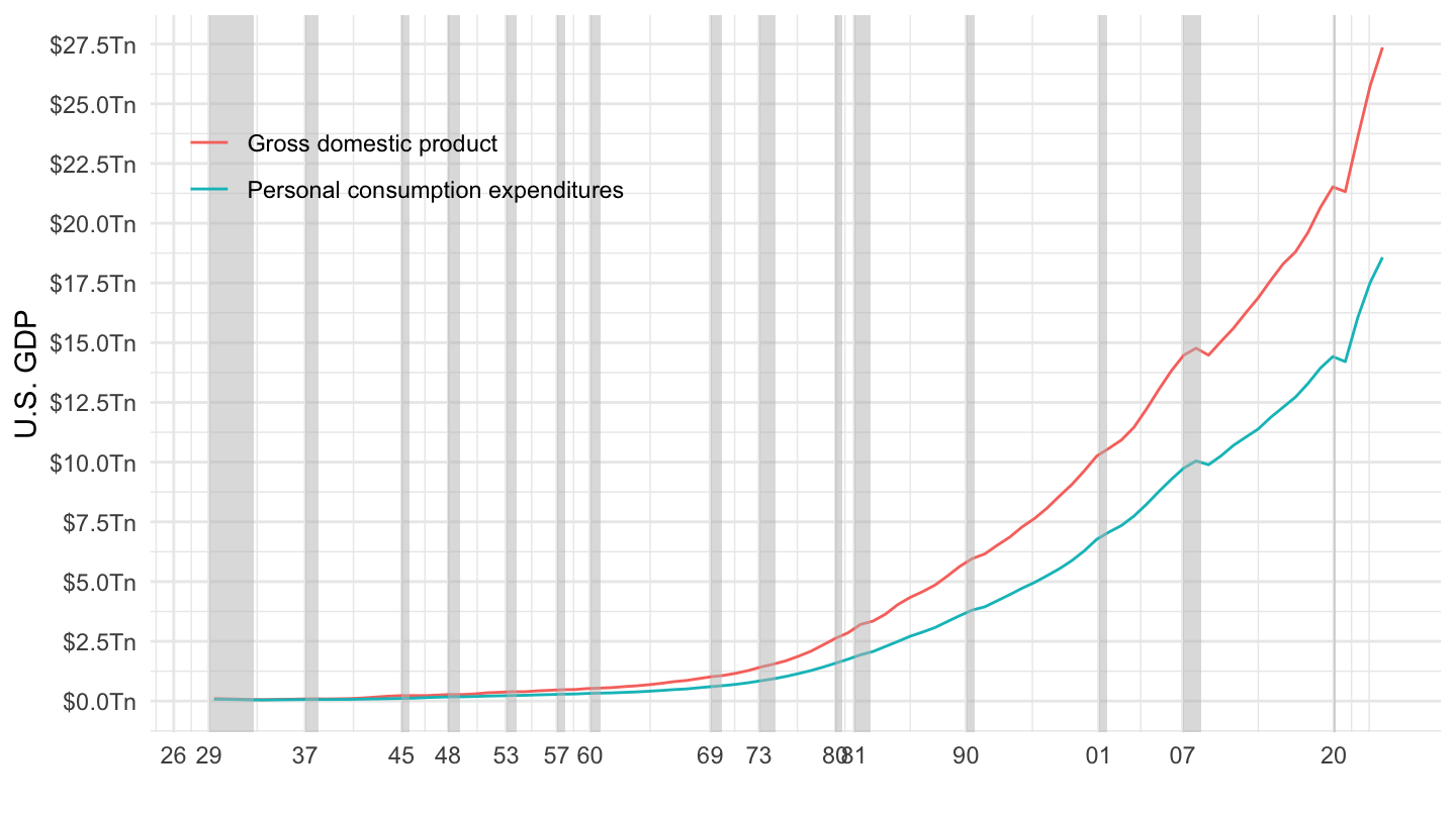
Log
Code
plot_log <- plot_linear +
  geom_rect(data = nber_recessions %>%
              filter(Peak > as.Date("1928-01-01")),
            aes(xmin = Peak, xmax = Trough, ymin = -Inf, ymax = +Inf),
            fill = 'grey', alpha = 0.5) +
  scale_y_log10(breaks = c(0.1, 0.2, 0.5, 1, 2, 5, 8, 10, 20),
                     labels = scales::dollar_format(accuracy = 0.1, suffix = "Tn"))

plot_log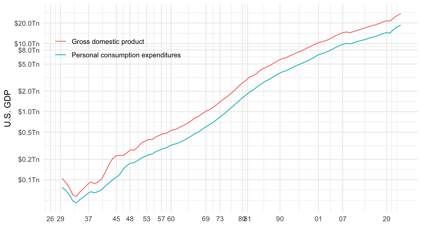
Both
Code
ggpubr::ggarrange(plot_linear + ggtitle("Linear Scale"),
                  plot_log + ggtitle("Log Scale") + ylab(""),
                  common.legend = T)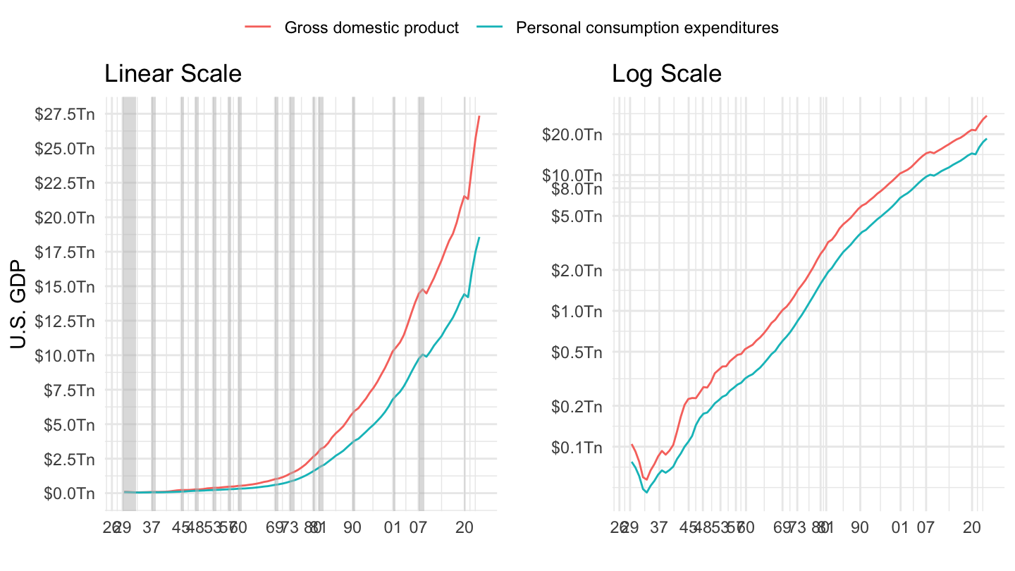
U.S. GDP (1929-2019)
(ref:gdp-only) U.S. GDP (1929-2019).
Code
T10105_A %>%
  year_to_date %>%
  filter(LineNumber == 1) %>%
  ggplot(.) + xlab("") + ylab("U.S. GDP") +
  geom_line(aes(x = date, y = DataValue/1000000)) +
  theme_minimal() +
  geom_rect(data = nber_recessions %>%
              filter(Peak > as.Date("1928-01-01")),
            aes(xmin = Peak, xmax = Trough, ymin = -Inf, ymax = +Inf),
            fill = 'grey', alpha = 0.5) +
  theme(legend.title = element_blank(),
        legend.position = c(0.2, 0.8)) +
  scale_x_date(breaks = nber_recessions$Peak,
               labels = date_format("%Y")) +
  scale_y_continuous(breaks = 1*seq(0, 40, 2.5),
                     labels = scales::dollar_format(accuracy = 0.1, suffix = "Tn"))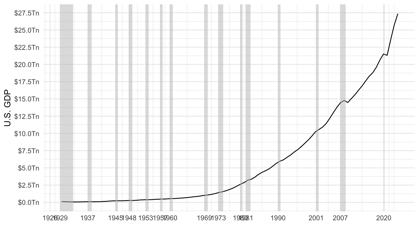
U.S. GDP (1929-2019) - Log Scale
(ref:log-gdp-only) U.S. GDP (1929-2019) - Log Scale.
Code
T10105_A %>%
  year_to_date %>%
  filter(LineNumber == 1) %>%
  ggplot(.) + xlab("") + ylab("U.S. GDP (Log Scale)") +
  geom_line(aes(x = date, y = DataValue/1000000)) + theme_minimal() +
  geom_rect(data = nber_recessions %>%
              filter(Peak > as.Date("1928-01-01")),
            aes(xmin = Peak, xmax = Trough, ymin = 0, ymax = +Inf),
            fill = 'grey', alpha = 0.5) +
  theme(legend.title = element_blank(),
        legend.position = c(0.2, 0.8)) +
  scale_x_date(breaks = nber_recessions$Peak,
               labels = date_format("%Y")) +
  scale_y_log10(breaks = 20*2^seq(-9, 1, 1),
                labels = scales::dollar_format(accuracy = 0.1, suffix = "Tn"))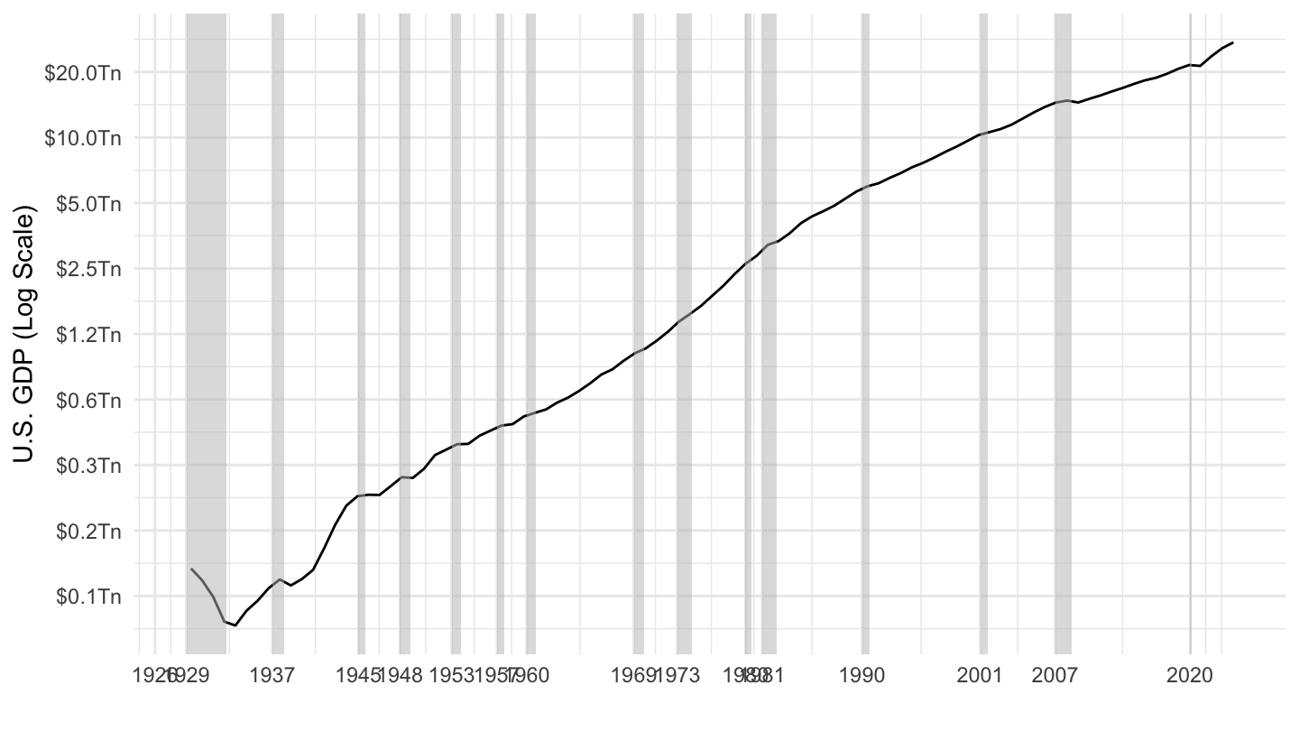
Government Purchases
HP Filter
(ref:g-purchases) Government Purchases.
Code
T10105_A %>%
  year_to_date %>%
  filter(LineNumber %in% c(1, 22)) %>%
  group_by(date) %>%
  summarise(government_gdp = DataValue[LineNumber == 22]/DataValue[LineNumber == 1]) %>%
  select(date, government_gdp) %>%
  inner_join(gdp_real_A, by = "date") %>%
  mutate(year = year(date),
         gdp_real_A_hp10000 = exp(hpfilter(log(gdp_real_A), freq = 10000)$trend),
         gdp_real_A_LLtrend = lm(log(gdp_real_A) ~ year) %>% fitted %>% exp) %>%
  transmute(date,
            `Government Purchases (% of GDP)` = government_gdp,
            `Government Purchases (% of Log-Linear GDP Trend)` = government_gdp * gdp_real_A / gdp_real_A_LLtrend,
            `Government Purchases (% of HP GDP Trend)` = government_gdp * gdp_real_A / gdp_real_A_hp10000) %>%
  gather(variable, value, -date) %>%
  ggplot(.) + geom_line(aes(x = date, y = value, color = variable, linetype = variable)) + theme_minimal() +
  theme(legend.title = element_blank(),
        legend.position = c(0.4, 0.15)) +
  scale_color_manual(values = viridis(4)[1:3]) +
  geom_rect(data = nber_recessions %>%
              filter(Peak > as.Date("1928-01-01")),
            aes(xmin = Peak, xmax = Trough, ymin = -Inf, ymax = +Inf),
            fill = 'grey', alpha = 0.5) +
  scale_x_date(breaks = nber_recessions$Peak,
               labels = date_format("%Y"),
               limits = as.Date(paste0(c(1947, 2019), "-01-01"))) +
  scale_y_continuous(breaks = seq(0.12, 0.29, 0.01),
                     labels = scales::percent_format(accuracy = 1),
                     limits = c(0.12, 0.29)) +
  xlab("") + ylab("Government Purchases (% of GDP)")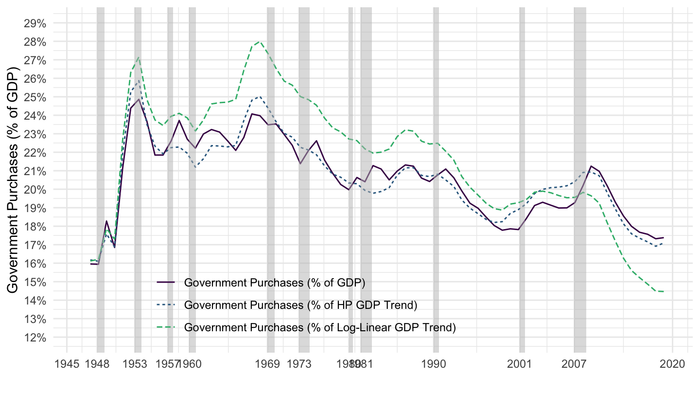
Residential investment
Code
T10105_A %>%
  year_to_date %>%
  filter(LineNumber %in% c(1, 13)) %>%
  group_by(date) %>%
  summarise(government_gdp = DataValue[LineNumber == 13]/DataValue[LineNumber == 1]) %>%
  select(date, government_gdp) %>%
  inner_join(gdp_real_A, by = "date") %>%
  mutate(year = year(date),
         gdp_real_A_hp10000 = log(gdp_real_A) %>% hpfilter(freq = 10000) %>% pluck("trend") %>% exp,
         gdp_real_A_LLtrend = lm(log(gdp_real_A) ~ year) %>% fitted %>% exp) %>%
  transmute(date,
            `Residential Investment (% of GDP)` = government_gdp,
            `Residential Investment (% of Log-Linear GDP Trend)` = government_gdp * gdp_real_A / gdp_real_A_LLtrend,
            `Residential Investment (% of HP GDP Trend)` = government_gdp * gdp_real_A / gdp_real_A_hp10000) %>%
  gather(variable, value, -date) %>%
  ggplot(.) + geom_line(aes(x = date, y = value, color = variable, linetype = variable)) + theme_minimal() +
  theme(legend.title = element_blank(),
        legend.position = c(0.4, 0.15)) +
  scale_color_manual(values = viridis(4)[1:3]) +
  geom_rect(data = nber_recessions %>%
              filter(Peak > as.Date("1928-01-01")),
            aes(xmin = Peak, xmax = Trough, ymin = -Inf, ymax = +Inf),
            fill = 'grey', alpha = 0.5) +
  scale_x_date(breaks = nber_recessions$Peak,
               labels = date_format("%Y"),
               limits = as.Date(paste0(c(1947, 2019), "-01-01"))) +
  scale_y_continuous(breaks = seq(0, 0.29, 0.01),
                     labels = scales::percent_format(accuracy = 1)) +
  xlab("") + ylab("Government Purchases (% of GDP)")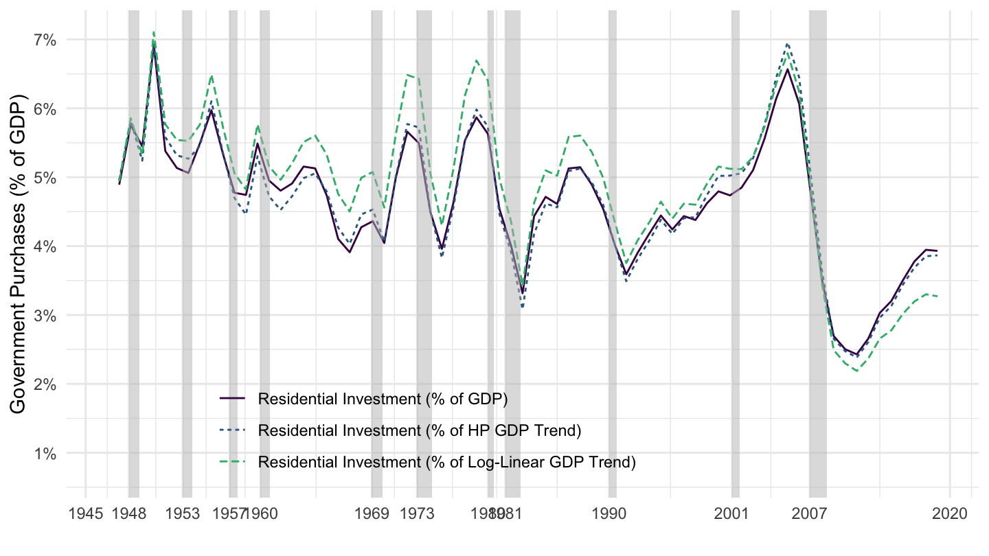
Net Exports
HP Filter
Code
T10105_A %>%
  year_to_date %>%
  filter(LineNumber %in% c(1, 15)) %>%
  group_by(date) %>%
  summarise(net_exports_gdp = DataValue[LineNumber == 15]/DataValue[LineNumber == 1]) %>%
  select(date, net_exports_gdp) %>%
  inner_join(gdp_real_A, by = "date") %>%
  mutate(year = year(date),
         gdp_real_A_hp10000 = log(gdp_real_A) %>% hpfilter(freq = 10000) %>% pluck("trend") %>% exp,
         gdp_real_A_LLtrend = lm(log(gdp_real_A) ~ year) %>% fitted %>% exp) %>%
  transmute(date,
            `Net Exports (% of GDP)` = net_exports_gdp,
            `Net Exports (% of Log-Linear GDP Trend)` = net_exports_gdp * gdp_real_A / gdp_real_A_LLtrend,
            `Net Exports (% of HP GDP Trend)` = net_exports_gdp * gdp_real_A / gdp_real_A_hp10000) %>%
  gather(variable, value, -date) %>%
  ggplot(.) + theme_minimal() + xlab("") + ylab("Net Exports (% of GDP)") +
  geom_line(aes(x = date, y = value, color = variable, linetype = variable)) +
  geom_hline(yintercept = 0, linetype = "dashed",  color = "black") +
  scale_color_manual(values = viridis(4)[1:3]) +
  theme(legend.title = element_blank(),
        legend.position = c(0.75, 0.85)) +
  scale_x_date(breaks = seq(1920, 2100, 5) %>% paste0("-01-01") %>% as.Date,
               labels = date_format("%Y")) +
  scale_y_continuous(breaks = seq(-0.06, 0.05, 0.01),
                     labels = scales::percent_format(accuracy = 1))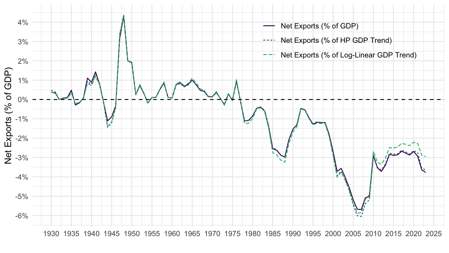
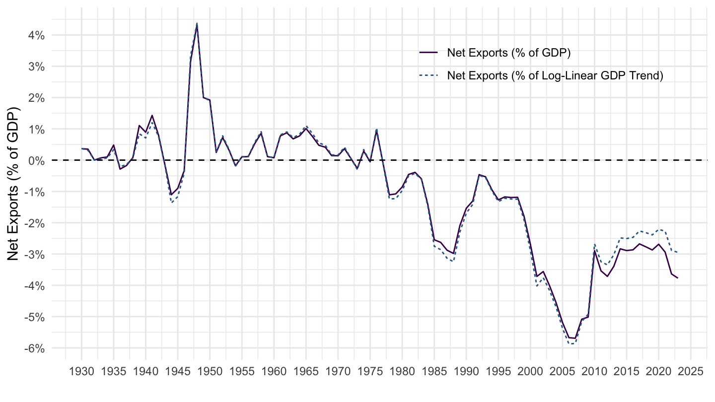
No HP Filter
Code
T10105_A %>%
  year_to_date %>%
  filter(LineNumber %in% c(1, 15)) %>%
  group_by(date) %>%
  summarise(net_exports_gdp = DataValue[LineNumber == 15]/DataValue[LineNumber == 1]) %>%
  select(date, net_exports_gdp) %>%
  inner_join(gdp_real_A, by = "date") %>%
  mutate(year = year(date),
         gdp_real_A_LLtrend = exp(fitted(lm(log(gdp_real_A) ~ year)))) %>%
  transmute(date,
            `Net Exports (% of GDP)` = net_exports_gdp,
            `Net Exports (% of Log-Linear GDP Trend)` = net_exports_gdp * gdp_real_A / gdp_real_A_LLtrend) %>%
  gather(variable, value, -date) %>%
  ggplot(.) + theme_minimal() + xlab("") + ylab("Net Exports (% of GDP)") +
  geom_line(aes(x = date, y = value, color = variable, linetype = variable)) +
  geom_hline(yintercept = 0, linetype = "dashed",  color = "black") +
  scale_color_manual(values = viridis(4)[1:3]) +
  theme(legend.title = element_blank(),
        legend.position = c(0.75, 0.85)) +
  scale_x_date(breaks = seq(1920, 2100, 5) %>% paste0("-01-01") %>% as.Date,
               labels = date_format("%Y")) +
  scale_y_continuous(breaks = seq(-0.06, 0.05, 0.01),
                     labels = scales::percent_format(accuracy = 1))