
Last observation: Q2 2026 (N = 27) · 2025 (N = 27)
First observation: 1929 (N = 8) · Q1 1947 (N = 8)
Last data update: 24 oct. 2026, 00:05
Last compile: 24 oct. 2026, 00:09
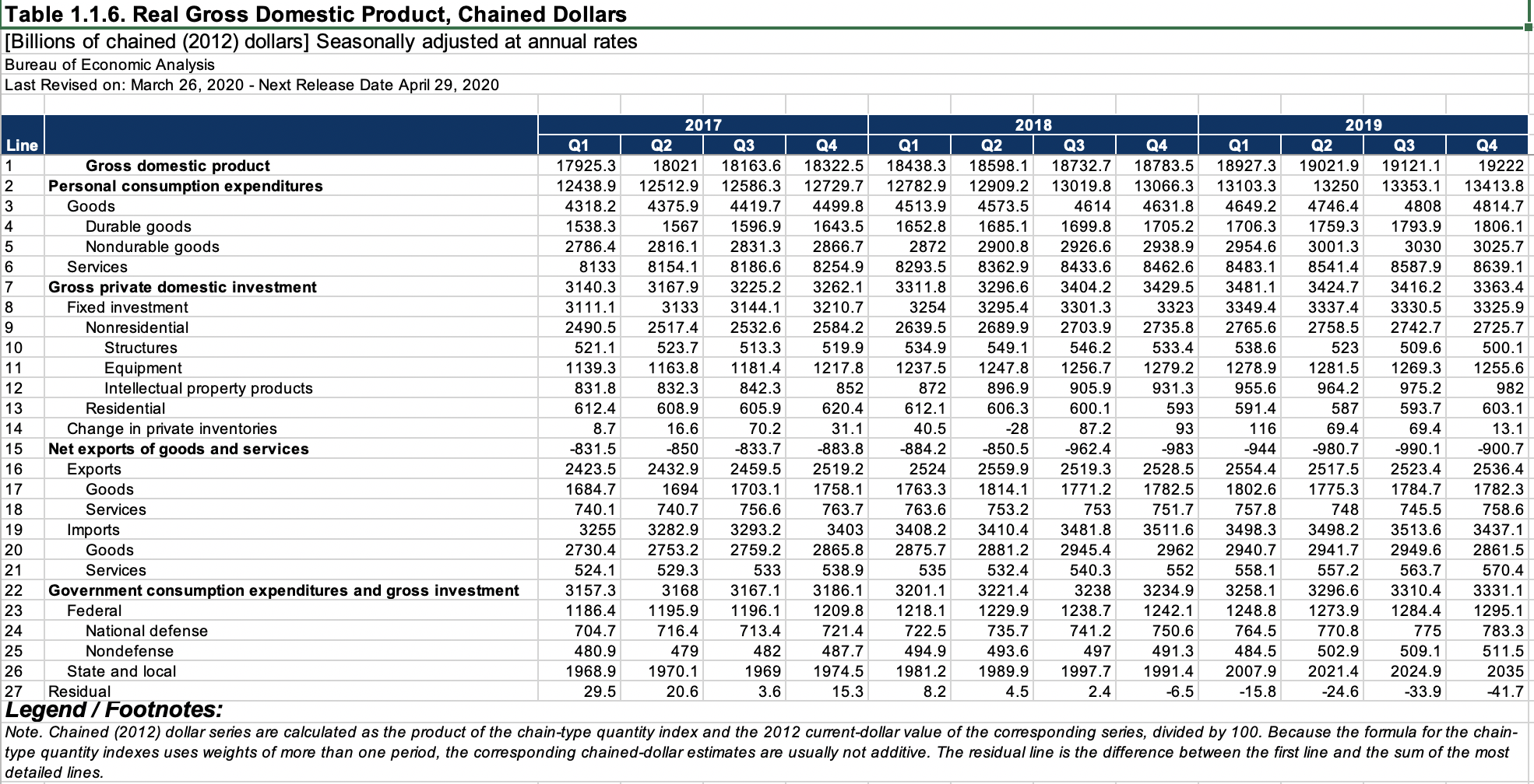
plot_linear <- T10106 |> filter(FREQ == "A") |>
  year_to_date() |>
  filter(LineNumber == 1) |>
  ggplot() + xlab("") + ylab("U.S. Real GDP") +
  geom_line(aes(x = date, y = DataValue/1000000)) +
  theme_minimal() +
  scale_x_date(breaks = nber_recessions$Peak,
               labels = date_format("%Y")) +
  scale_y_continuous(breaks = 1*seq(0, 50, 2.5),
                     labels = scales::dollar_format(accuracy = 0.1, suffix = "Tn")) +
  geom_rect(data = nber_recessions |>
              filter(Peak > as.Date("1928-01-01")),
            aes(xmin = Peak, xmax = Trough, ymin = 0, ymax = +Inf),
            fill = 'grey', alpha = 0.5)

plot_linear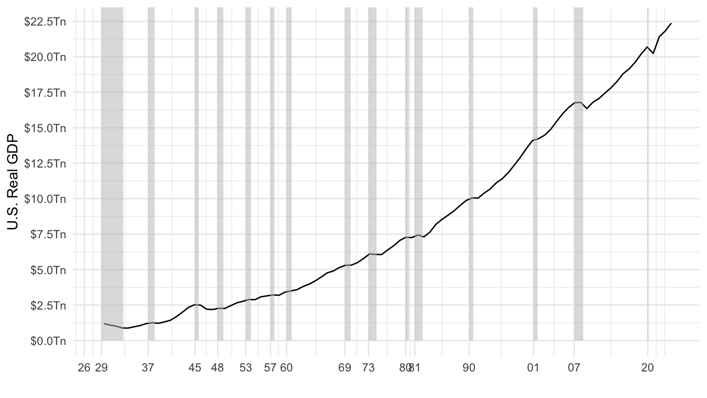
plot_log <- plot_linear +
  scale_y_log10(breaks = 20*2^seq(-7, 1, 1),
                labels = scales::dollar_format(accuracy = 0.1, suffix = "Tn")) +
  geom_rect(data = nber_recessions |>
              filter(Peak > as.Date("1928-01-01")),
            aes(xmin = Peak, xmax = Trough, ymin = 0, ymax = +Inf),
            fill = 'grey', alpha = 0.5)

plot_log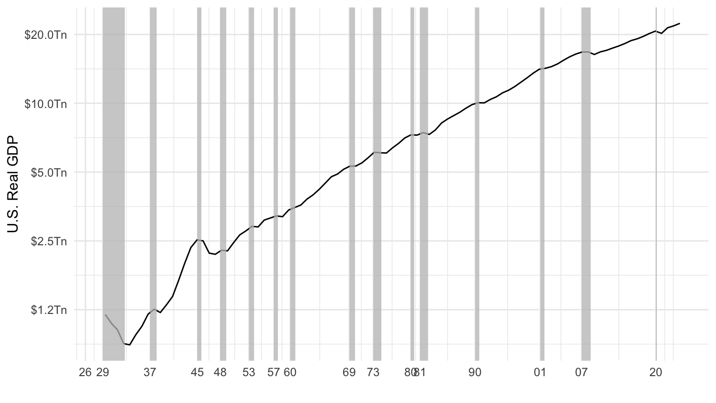
ggpubr::ggarrange(plot_linear + ggtitle("Linear Scale"), plot_log + ggtitle("Log Scale"))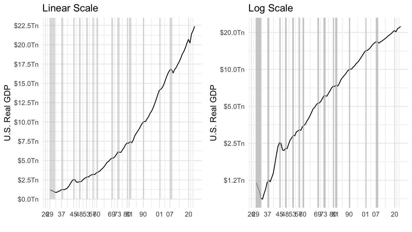
T10106 |> filter(FREQ == "Q") |>
  quarter_to_date() |>
  filter(LineNumber == 1) |>
  ggplot() + xlab("") + ylab("U.S. Real GDP") +
  geom_line(aes(x = date, y = DataValue/1000000)) +
  theme_minimal() +
  scale_x_date(breaks = nber_recessions$Peak,
               labels = date_format("%Y")) +
  scale_y_log10(breaks = 20*2^seq(-7, 1, 1),
                labels = scales::dollar_format(accuracy = 0.1, suffix = "Tn")) +
  geom_rect(data = nber_recessions |>
              filter(Peak > as.Date("1945-01-01")),
            aes(xmin = Peak, xmax = Trough, ymin = 0, ymax = +Inf),
            fill = 'grey', alpha = 0.5)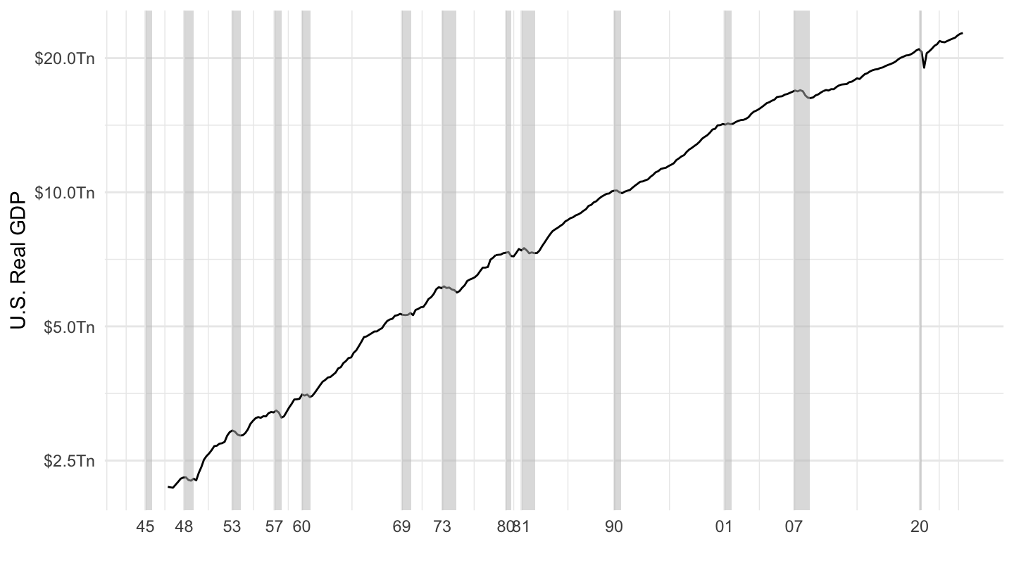
T10106 |> filter(FREQ == "Q") |>
  quarter_to_date() |>
  filter(LineNumber == 1,
         date >= as.Date("1970-01-01")) |>
  ggplot() + xlab("") + ylab("U.S. Real GDP") +
  geom_line(aes(x = date, y = DataValue/1000000)) +
  theme_minimal() +
  scale_x_date(breaks = c(nber_recessions$Peak),
               labels = date_format("%Y")) +
  scale_y_log10(breaks = 20*2^seq(-7, 1, 0.2),
                labels = scales::dollar_format(accuracy = 0.1, suffix = "Tn")) +
  geom_rect(data = nber_recessions |>
              filter(Peak > as.Date("1970-01-01")),
            aes(xmin = Peak, xmax = Trough, ymin = 0, ymax = +Inf),
            fill = 'grey', alpha = 0.5)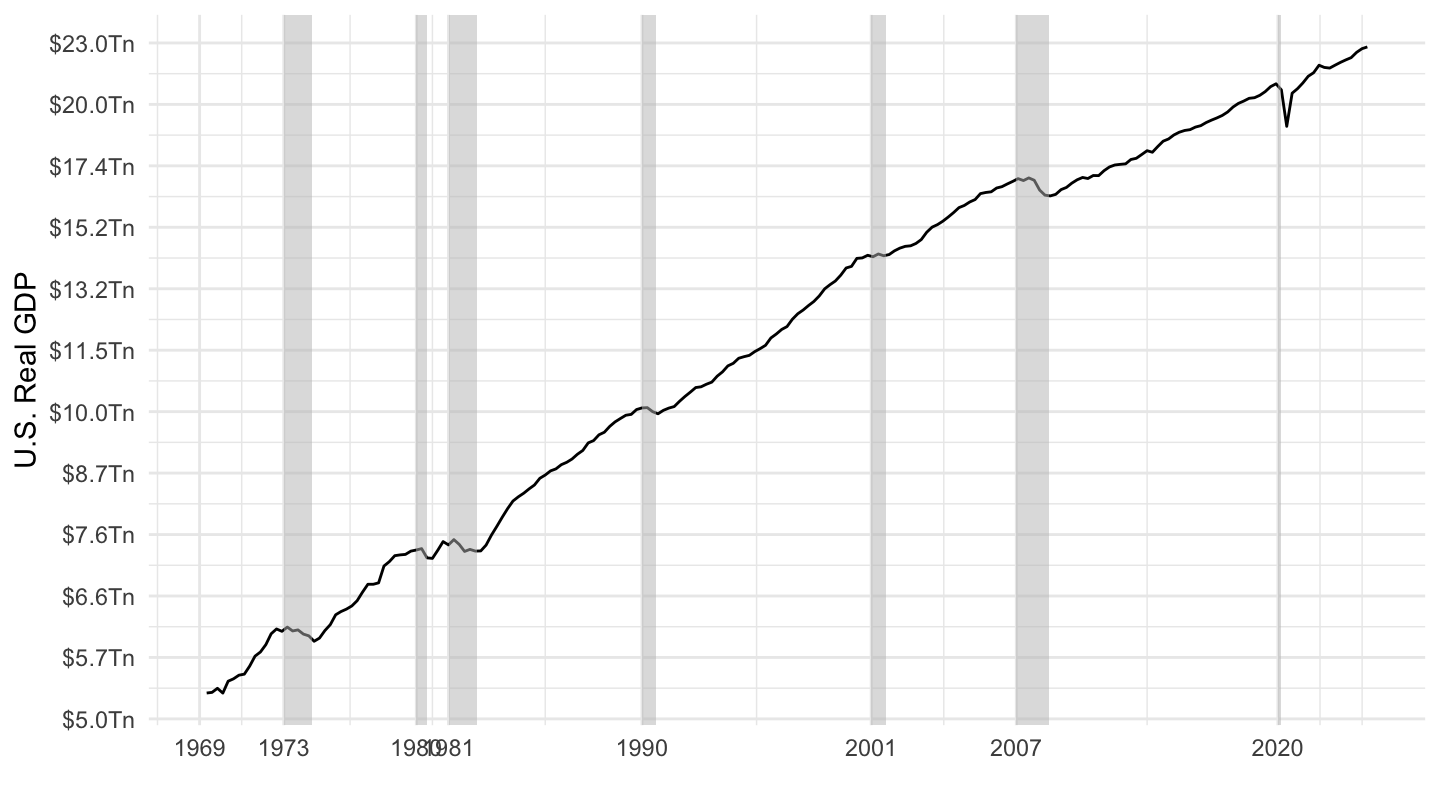
T10106 |> filter(FREQ == "Q") |>
  quarter_to_date() |>
  filter(LineNumber == 1,
         date >= as.Date("1990-01-01")) |>
  ggplot() + xlab("") + ylab("U.S. Real GDP") +
  geom_line(aes(x = date, y = DataValue/1000000)) +
  theme_minimal() +
  scale_x_date(breaks = c(nber_recessions$Peak),
               labels = date_format("%Y")) +
  scale_y_log10(breaks = 20*2^seq(-7, 1, 0.1),
                labels = scales::dollar_format(accuracy = 0.1, suffix = "Tn")) +
  geom_rect(data = nber_recessions |>
              filter(Peak > as.Date("1990-01-01")),
            aes(xmin = Peak, xmax = Trough, ymin = 0, ymax = +Inf),
            fill = 'grey', alpha = 0.5)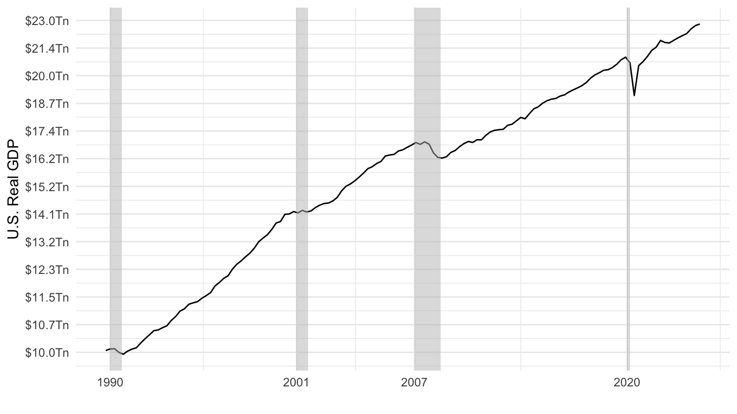
T10106 |> filter(FREQ == "Q") |>
  quarter_to_date() |>
  filter(LineNumber == 1,
         date >= as.Date("2005-01-01")) |>
  ggplot() + xlab("") + ylab("U.S. Real GDP") +
  geom_line(aes(x = date, y = DataValue/1000000)) +
  theme_minimal() +
  scale_x_date(breaks = "2 years",
               labels = date_format("%Y")) +
  scale_y_log10(breaks = 20*2^seq(-7, 1, .1),
                labels = scales::dollar_format(accuracy = 0.1, suffix = "Tn")) +
  geom_rect(data = nber_recessions |>
              filter(Peak > as.Date("2005-01-01")),
            aes(xmin = Peak, xmax = Trough, ymin = 0, ymax = +Inf),
            fill = 'grey', alpha = 0.5)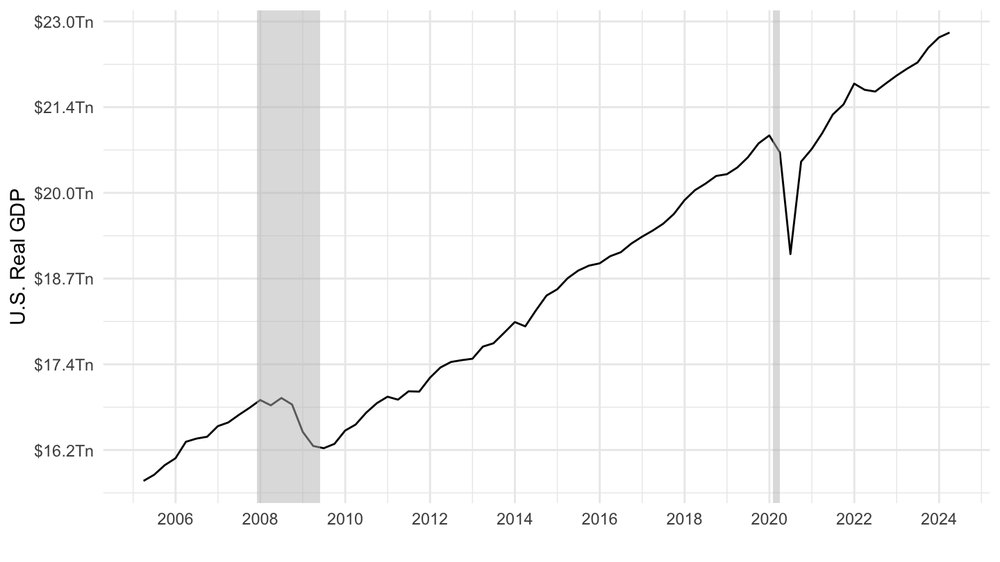
T10106 |> filter(FREQ == "A") |>
  year_to_date() |>
  filter(LineNumber == 1) |>
  select(date, `Real GDP` = DataValue) |>
  mutate(`Real GDP` = `Real GDP` / 1000000,
         year = year(date)) |>
  mutate(`HP (1000) Trend` = exp(hpfilter(log(`Real GDP`), freq = 1000, type = "lambda", drift = FALSE)$trend),
         `HP (10000) Trend` = exp(hpfilter(log(`Real GDP`), freq = 10000, type = "lambda", drift = FALSE)$trend),
         `Log-Linear Trend` = exp(fitted(lm(log(`Real GDP`) ~ year, na.action = na.exclude)))) |>
  group_by(date) |>
  select(-year) |>
  gather(variable, value, -date) |>
  ggplot() + geom_line(aes(x = date, y = value, color = variable, linetype = variable)) +
  theme_minimal() +
  scale_color_manual(values = viridis(5)[1:4]) +
  theme(legend.title = element_blank(),
        legend.position = c(0.8, 0.2)) +
  scale_x_date(breaks = nber_recessions$Peak,
               labels = date_format("%Y")) +
  scale_y_log10(breaks = 20*2^seq(-7, 1, 1),
                labels = scales::dollar_format(accuracy = 0.1, suffix = "Tn")) +
  geom_rect(data = nber_recessions |>
              filter(Peak > as.Date("1928-01-01")),
            aes(xmin = Peak, xmax = Trough, ymin = 0, ymax = +Inf),
            fill = 'grey', alpha = 0.5) +
  xlab("") + ylab("U.S. Real GDP")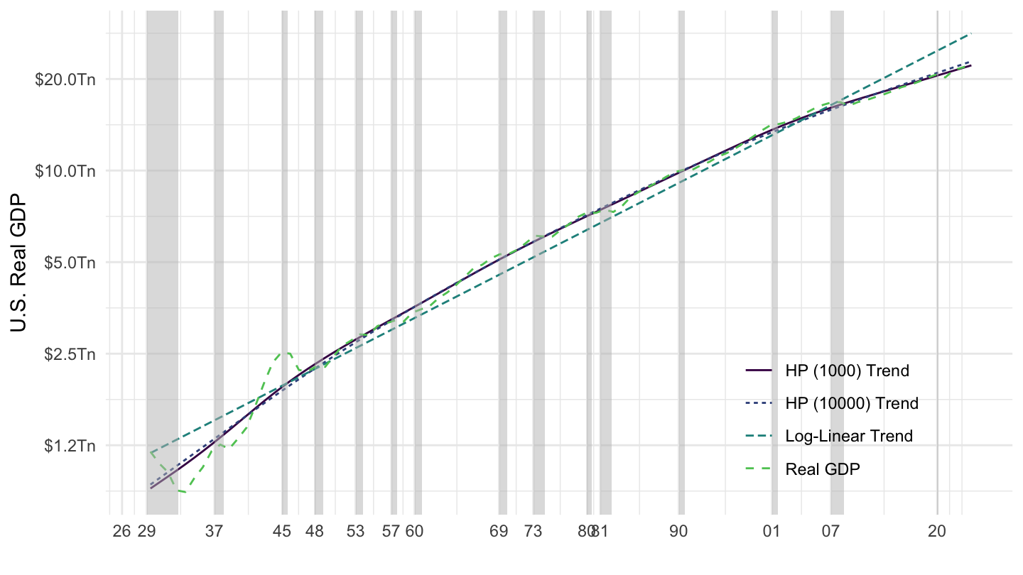
T10106 |> filter(FREQ == "A") |>
  year_to_date() |>
  filter(LineNumber == 1) |>
  select(date, `Real GDP` = DataValue) |>
  mutate(`Real GDP` = `Real GDP` / 1000000,
         year = year(date)) |>
  mutate(`HP (1000) Cycle` = exp(hpfilter(log(`Real GDP`), freq = 1000, type = "lambda", drift = FALSE)$cycle),
         `HP (10000) Cycle` = exp(hpfilter(log(`Real GDP`), freq = 10000, type = "lambda", drift = FALSE)$cycle),
         `Log-Linear Cycle` = exp(residuals(lm(log(`Real GDP`) ~ year, na.action = na.exclude)))) |>
  group_by(date) |>
  select(-year, - `Real GDP`) |>
  gather(variable, value, -date) |>
  ggplot() + geom_line(aes(x = date, y = value, color = variable, linetype = variable)) + theme_minimal() +
  theme(legend.title = element_blank(),
        legend.position = c(0.8, 0.8)) +
  geom_rect(data = nber_recessions |>
              filter(Peak > as.Date("1928-01-01")),
            aes(xmin = Peak, xmax = Trough, ymin = -Inf, ymax = +Inf),
            fill = 'grey', alpha = 0.5) +
  scale_x_date(breaks = nber_recessions$Peak,
               labels = date_format("%Y")) +
  scale_y_continuous(breaks = seq(0.60, 1.40, 0.05),
                     labels = scales::percent_format(accuracy = 1)) +
  xlab("") + ylab("GDP Cycle (% of Trend)")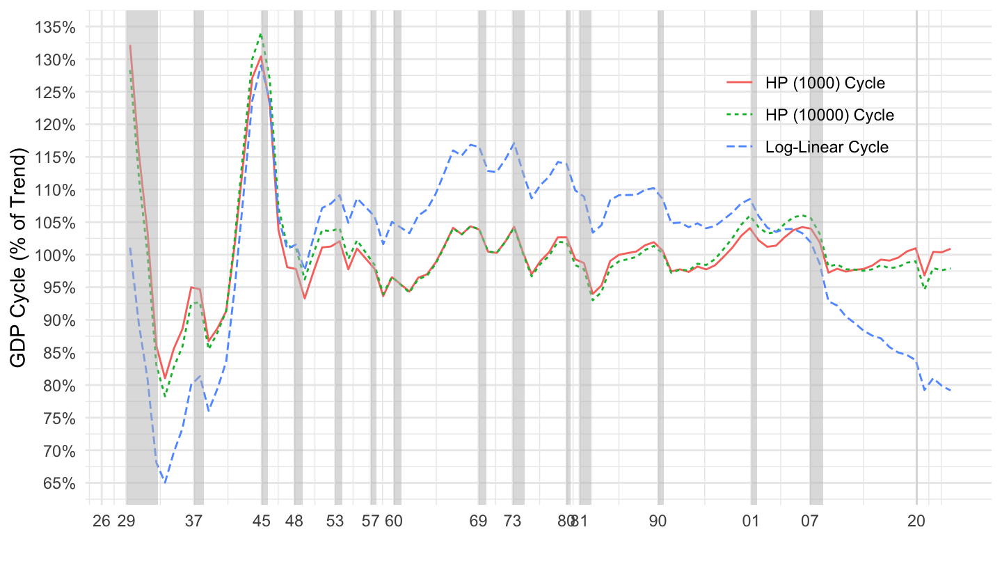
fit <- T10106 |> filter(FREQ == "A") |>
  year_to_date() |>
  filter(LineNumber == 1) |>
  select(date, `Real GDP` = DataValue) |>
  mutate(`Real GDP` = `Real GDP` / 1000000,
         year = year(date)) |>
  filter(year <= 1971) %>%
  lm(log(`Real GDP`) ~ year, data = .) |>
  pluck("coefficients")

fit_2019 <- T10106 |> filter(FREQ == "A") |>
  year_to_date() |>
  filter(LineNumber == 1) |>
  select(date, `Real GDP` = DataValue) |>
  mutate(`Real GDP` = `Real GDP` / 1000000,
         year = year(date)) %>%
  lm(log(`Real GDP`) ~ year, data = .) |>
  pluck("coefficients")

fit_1929_1971 <- T10106 |> filter(FREQ == "A") |>
  year_to_date() |>
  filter(LineNumber == 1) |>
  select(date, `Real GDP` = DataValue) |>
  mutate(`Real GDP` = `Real GDP` / 1000000,
         year = year(date)) |>
  filter(year <= 1971) %>%
  lm(log(`Real GDP`) ~ year, data = .) |>
  pluck("coefficients")

fit_1929_1971
# (Intercept) year
# -83.52871738 0.04327969fit_1972_2019 <- T10106 |> filter(FREQ == "A") |>
year_to_date() |>
filter(LineNumber == 1) |>
select(date, `Real GDP` = DataValue) |>
mutate(`Real GDP` = `Real GDP` / 1000000,
year = year(date)) |>
filter(year >= 1972) %>%
lm(log(`Real GDP`) ~ year, data = .) |>
pluck("coefficients")(ref:us-log-real-gdp-nipa-trend) U.S. Real GDP Trends (1929-2019) - Log Scale.
T10106 |> filter(FREQ == "A") |>
  year_to_date() |>
  filter(LineNumber == 1) |>
  select(date, `Real GDP` = DataValue) |>
  mutate(`Real GDP` = `Real GDP` / 1000000,
         year = year(date)) |>
  mutate(`Trend to 2019 (g = 3.5%)` = lm(log(`Real GDP`) ~ year) |> fitted() |> exp(),
         `Trend to 1971, extrapolated` = ifelse(year >= 1971, (fit[1] + fit[2] * year) |> exp(), NA),
         `Trend to 1971 (g = 4.1%)` = ifelse(year <= 1971, (fit[1] + fit[2] * year) |> exp(), NA)) |>
  group_by(date) |>
  select(-year) |>
  gather(variable, value, -date) |>
  ggplot() + geom_line(aes(x = date, y = value, color = variable, linetype = variable)) +
  theme_minimal() +
  scale_color_manual(values = c(viridis(4)[3], viridis(4)[1], viridis(4)[1], viridis(4)[2])) +
  scale_linetype_manual(values = c("solid", "solid", "dashed", "solid")) +
  theme(legend.title = element_blank(),
        legend.position = c(0.8, 0.2)) +
  scale_x_date(breaks = nber_recessions$Peak,
               labels = date_format("%Y")) +
  scale_y_log10(breaks = 20*2^seq(-7, 1, 1),
                labels = scales::dollar_format(accuracy = 0.1, suffix = "Tn")) +
  geom_rect(data = nber_recessions |>
              filter(Peak > as.Date("1928-01-01")),
            aes(xmin = Peak, xmax = Trough, ymin = 0, ymax = +Inf),
            fill = 'grey', alpha = 0.5) +
  xlab("") + ylab("U.S. Real GDP, $2012")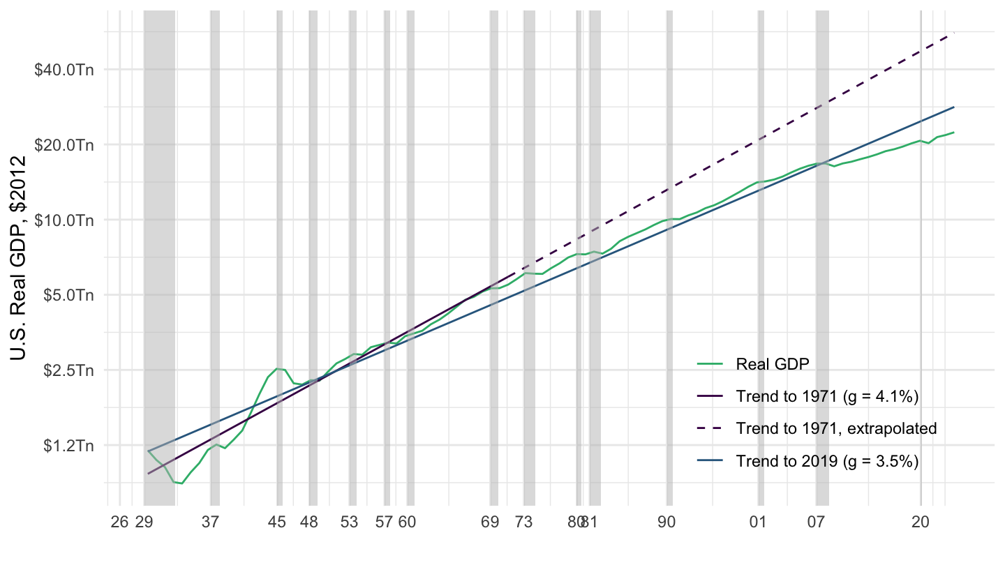
(ref:us-real-gdp-nipa-trend) U.S. Real GDP Trends (1929-2019).
T10106 |> filter(FREQ == "A") |>
  year_to_date() |>
  filter(LineNumber == 1) |>
  select(date, `Real GDP` = DataValue) |>
  mutate(`Real GDP` = `Real GDP` / 1000000,
         year = year(date)) |>
  mutate(`Trend to 2019 (g = 3.5%)` = lm(log(`Real GDP`) ~ year) |> fitted() |> exp(),
         `Trend to 1971, extrapolated` = ifelse(year >= 1971, (fit[1] + fit[2] * year) |> exp(), NA),
         `Trend to 1971 (g = 4.1%)` = ifelse(year <= 1971, (fit[1] + fit[2] * year) |> exp(), NA)) |>
  group_by(date) |>
  select(-year) |>
  gather(variable, value, -date) |>
  ggplot() + geom_line(aes(x = date, y = value, color = variable, linetype = variable)) +
  theme_minimal() +
  scale_color_manual(values = c(viridis(4)[3], viridis(4)[1], viridis(4)[1], viridis(4)[2])) +
  scale_linetype_manual(values = c("solid", "solid", "dashed", "solid")) +
  theme(legend.title = element_blank(),
        legend.position = c(0.2, 0.8)) +
  scale_x_date(breaks = nber_recessions$Peak,
               labels = date_format("%Y")) +
  scale_y_continuous(breaks = 20*2^seq(-4, 1, 1),
                labels = scales::dollar_format(accuracy = 0.1, suffix = "Tn")) +
  geom_rect(data = nber_recessions |>
              filter(Peak > as.Date("1928-01-01")),
            aes(xmin = Peak, xmax = Trough, ymin = 0, ymax = +Inf),
            fill = 'grey', alpha = 0.5) +
  xlab("") + ylab("U.S. Real GDP, $2012")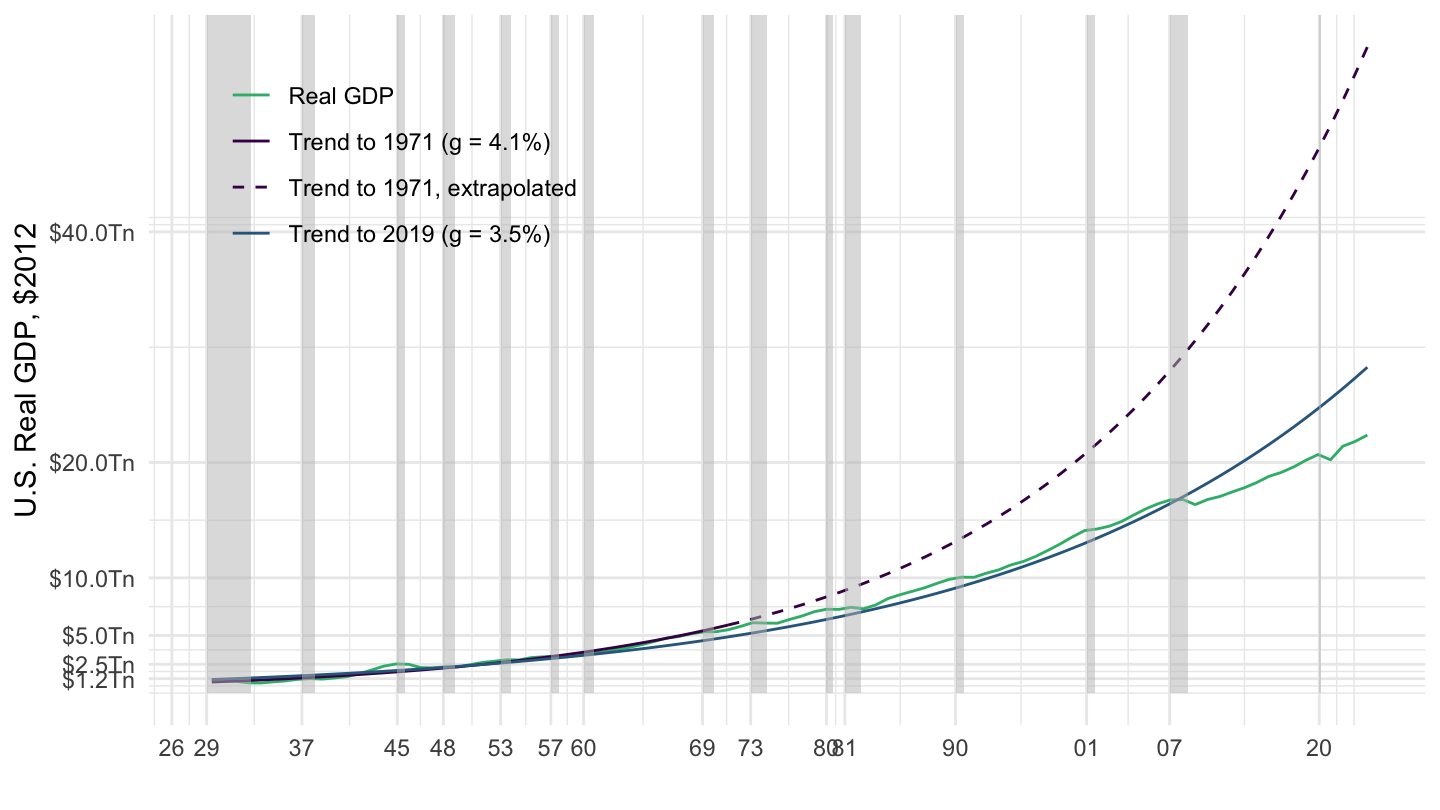
(ref:us-real-gdp-nipa-cycle) U.S. Real GDP Cycles (1929-2019).
T10106 |> filter(FREQ == "A") |>
  year_to_date() |>
  filter(LineNumber == 1) |>
  select(date, `Real GDP` = DataValue) |>
  mutate(`Real GDP` = `Real GDP` / 1000000,
         year = year(date)) |>
  mutate(`Cycle, Detrending to 2019 (g = 3.5%)` = lm(log(`Real GDP`) ~ year) |> residuals() |> exp(),
         `Cycle, Detrending to 1971, extrapolated` = ifelse(year >= 1971, exp(log(`Real GDP`) - fit[1] - fit[2] * year), NA),
         `Cycle, Detrending to 1971 (g = 4.1%)` = ifelse(year <= 1971, exp(log(`Real GDP`) - fit[1] - fit[2] * year), NA)) |>
  group_by(date) |>
  select(-year, -`Real GDP`) |>
  gather(variable, value, -date) |>
  ggplot() + geom_line(aes(x = date, y = value, color = variable, linetype = variable)) +
  theme_minimal() +
  scale_color_manual(values = c(viridis(4)[1],viridis(4)[1], viridis(4)[2])) +
  scale_linetype_manual(values = c("solid", "dashed", "solid")) +
  theme(legend.title = element_blank(),
        legend.position = c(0.7, 0.8)) +
  scale_x_date(breaks = nber_recessions$Peak,
               labels = date_format("%Y")) +
  scale_y_continuous(breaks = seq(0, 2.25, 0.10),
                labels = scales::percent_format(accuracy = 1),
                limits = c(0.4, 1.55)) +
  geom_rect(data = nber_recessions |>
              filter(Peak > as.Date("1928-01-01")),
            aes(xmin = Peak, xmax = Trough, ymin = -Inf, ymax = +Inf),
            fill = 'grey', alpha = 0.5) +
  xlab("") + ylab("U.S. Real GDP, $2012")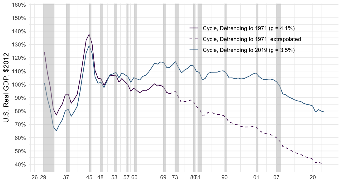
dataset <- T10106 |> filter(FREQ == "A") |>
  year_to_date() |>
  filter(LineNumber == 1) |>
  select(date, `Real GDP` = DataValue) |>
  mutate(`Real GDP` = `Real GDP` / 1000000,
         year = year(date)) |>
  select(year, `Real GDP`)

fit <- dataset |>
  filter(year <= 1971) %>%
  lm(log(`Real GDP`) ~ year, data = .) |>
  pluck("coefficients")

fit_2019 <- dataset %>%
  lm(log(`Real GDP`) ~ year, data = .) |>
  pluck("coefficients")

fit_1929_1971 <- dataset |>
  filter(year <= 1971) %>%
  lm(log(`Real GDP`) ~ year, data = .) |>
  pluck("coefficients")

fit_1972_2019 <- dataset |>
  filter(year >= 1972) %>%
  lm(log(`Real GDP`) ~ year, data = .) |>
pluck("coefficients")ssq1 <- dataset %>%
lm(log(`Real GDP`) ~ year, data = .) |>
pluck("residuals") |>
norm(type = "2")
ssq2 <- dataset |>
mutate(year2 = year^2) %>%
lm(log(`Real GDP`) ~ year + year2, data = .) |>
pluck("residuals") |>
norm(type = "2")
ssq3a <- dataset |>
filter(year >= 1972) %>%
lm(log(`Real GDP`) ~ year, data = .) |>
pluck("residuals") |>
norm(type = "2")
ssq3b <- dataset |>
filter(year <= 1971) %>%
lm(log(`Real GDP`) ~ year, data = .) |>
pluck("residuals") |>
norm(type = "2")
ssq1# [1] 1.394299ssq2# [1] 0.7942941ssq3a + ssq3b# [1] 1.139984T10106 |>
filter(FREQ == "A") |>
select(-FREQ) |>
year_to_date() |>
mutate(year = year(date)) |>
filter(year %in% c(1938, 1958, 1978, 1998, 2018)) |>
group_by(year) |>
mutate(value = round(100*DataValue/DataValue[1], 1)) |>
ungroup() |>
select(2, 3, 6, 7) |>
spread(year, value) %>%
{if (is_html_output()) datatable(., filter = 'top', rownames = F) else .}T10106 |> filter(FREQ == "A") |>
select(-FREQ) |>
year_to_date() |>
mutate(year = year(date)) |>
filter(year %in% c(1938, 1958, 1978, 1998, 2018)) |>
group_by(year) |>
mutate(value = round(DataValue/1000)) |>
ungroup() |>
select(2, 3, 6, 7) |>
spread(year, value) %>%
{if (is_html_output()) datatable(., filter = 'top', rownames = F) else .}| source | dataset | Title | Updated |
|---|---|---|---|
