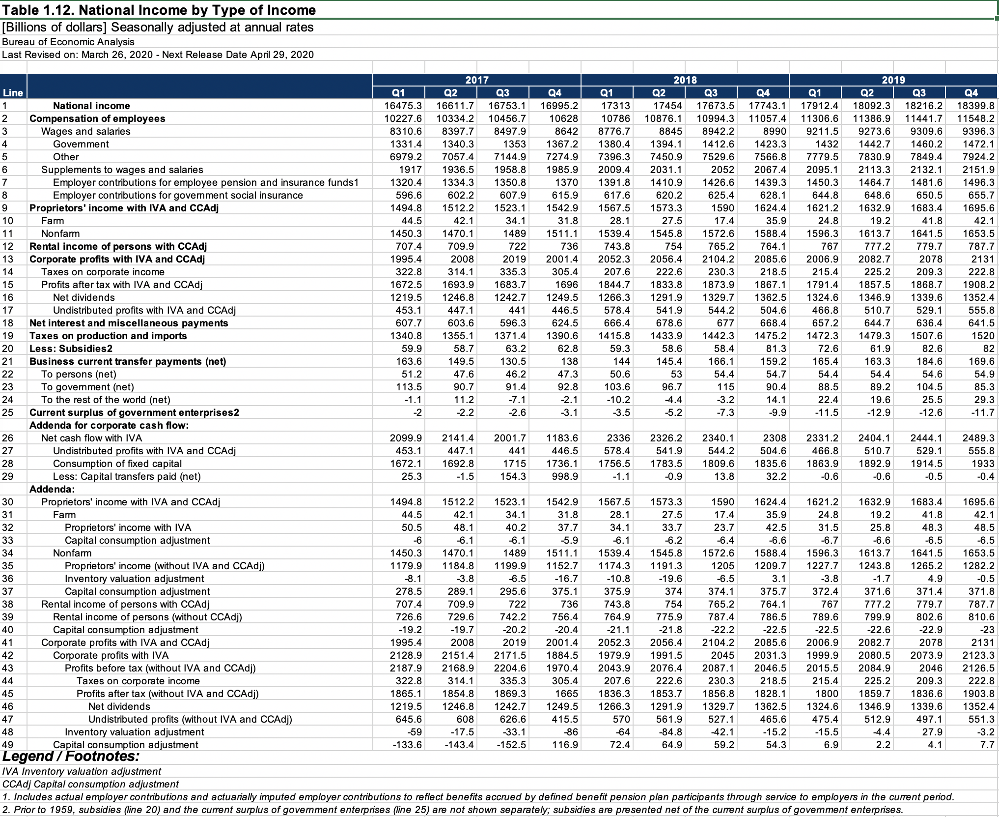
Table 1.12. National Income by Type of Income (A) (Q)

Data - BEA

~/data/bea/NIPA.html

Info

source	dataset	.html	.RData
bea	T10106	2024-02-11	2023-12-17
bea	T11200	2024-01-06	2023-12-17

Data on US macro

source	dataset	.html	.RData
fred	gdp	2024-02-03	2024-02-11
fred	unr	2024-02-03	2024-02-03
oecd	QNA	2024-01-28	2024-02-03
oecd	SNA_TABLE1	2024-01-28	2024-02-03

LAST_COMPILE

LAST_COMPILE
2024-02-11

Last

date	Nobs
2023-09-30	49

Layout

• NIPA Website. html

Replicating Abel et al. (1989)

Rents

1938, 1958, 1978, 1998, 2018 Table

Percent

T11200 %>% filter(FREQ == "A") %>% select(-FREQ) %>%
  year_to_date %>%
  mutate(year = year(date)) %>%
  filter(year %in% c(1938, 1958, 1978, 1998, 2018)) %>%
  group_by(year) %>%
  mutate(value = round(100*DataValue/DataValue[1], 1)) %>%
  ungroup %>%
  select(2, 3, 6, 7) %>%
  spread(year, value) %>%
  {if (is_html_output()) datatable(., filter = 'top', rownames = F) else .}

Percent - pdf

i_g("bib/bea/T11200.png")

Billions

T11200 %>% filter(FREQ == "A") %>% select(-FREQ) %>%
  year_to_date %>%
  mutate(year = year(date)) %>%
  filter(year %in% c(1938, 1958, 1978, 1998, 2018)) %>%
  group_by(year) %>%
  mutate(value = round(DataValue/1000)) %>%
  ungroup %>%
  select(2, 3, 6, 7) %>%
  spread(year, value) %>%
  {if (is_html_output()) datatable(., filter = 'top', rownames = F) else .}

Econ 102

Net dividends and undistributed profits

T11200 %>% filter(FREQ == "A") %>% select(-FREQ) %>%
  year_to_date %>%
  filter(LineNumber %in% c(1, 16, 15, 17)) %>%
  group_by(date) %>%
  summarise(`Net Dividends` = DataValue[LineNumber == 16]/DataValue[LineNumber == 1],
            `Profits after tax with IVA and CCAdj` = DataValue[LineNumber == 15]/DataValue[LineNumber == 1],
            `Undistributed profits with IVA and CCAdj` = DataValue[LineNumber == 17]/DataValue[LineNumber == 1]) %>%
  gather(variable, value, -date) %>%
  ggplot(.) + theme_minimal() + xlab("") + ylab("Profits (% of GDI)") +
  geom_line(aes(x = date, y = value, color = variable)) +
  theme(legend.title = element_blank(),
        legend.position = c(0.3, 0.85)) +
  geom_rect(data = nber_recessions %>%
              filter(Peak > as.Date("1928-01-01")), 
            aes(xmin = Peak, xmax = Trough, ymin = -Inf, ymax = +Inf), 
            fill = 'grey', alpha = 0.5) + 
  scale_x_date(breaks = nber_recessions$Peak,
               labels = date_format("%Y")) +
  scale_y_continuous(breaks = seq(0, 0.80, 0.01),
                     labels = scales::percent_format(accuracy = 1),
                     limits = c(0, 0.14))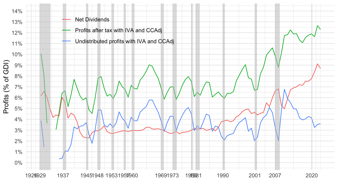

Compensation of Employees

T11200 %>% filter(FREQ == "A") %>% select(-FREQ) %>%
  year_to_date %>%
  filter(LineNumber %in% c(1, 2)) %>%
  group_by(date) %>%
  summarise(value_gdp = DataValue[LineNumber == 2]/DataValue[LineNumber == 1]) %>%
  select(date, value_gdp) %>%
  left_join(gdp_real_A, by = "date") %>%
  mutate(year = year(date),
         gdp_real_A_hp10000 = log(gdp_real_A) %>% hpfilter(freq = 10000) %>% pluck("trend") %>% exp,
         gdp_real_A_LLtrend = lm(log(gdp_real_A) ~ year) %>% fitted %>% exp) %>%
  transmute(date,
            `Compensation of Employees (% of GDI)` = value_gdp,
            `Compensation of Employees (% of Log-Linear GDI Trend)` = value_gdp * gdp_real_A / gdp_real_A_LLtrend,
            `Compensation of Employees (% of HP GDI Trend)` = value_gdp * gdp_real_A / gdp_real_A_hp10000) %>%
  gather(variable, value, -date) %>%
  ggplot(.) + theme_minimal() + xlab("") + ylab("Compens. of Employees (% of GDI)") +
  geom_line(aes(x = date, y = value, color = variable)) +
  theme(legend.title = element_blank(),
        legend.position = c(0.5, 0.2)) +
  geom_rect(data = nber_recessions %>%
              filter(Peak > as.Date("1928-01-01")), 
            aes(xmin = Peak, xmax = Trough, ymin = -Inf, ymax = +Inf), 
            fill = 'grey', alpha = 0.5) + 
  scale_x_date(breaks = nber_recessions$Peak,
               labels = date_format("%Y")) +
  scale_y_continuous(breaks = seq(0.4, 0.80, 0.05),
                     labels = scales::percent_format(accuracy = 1))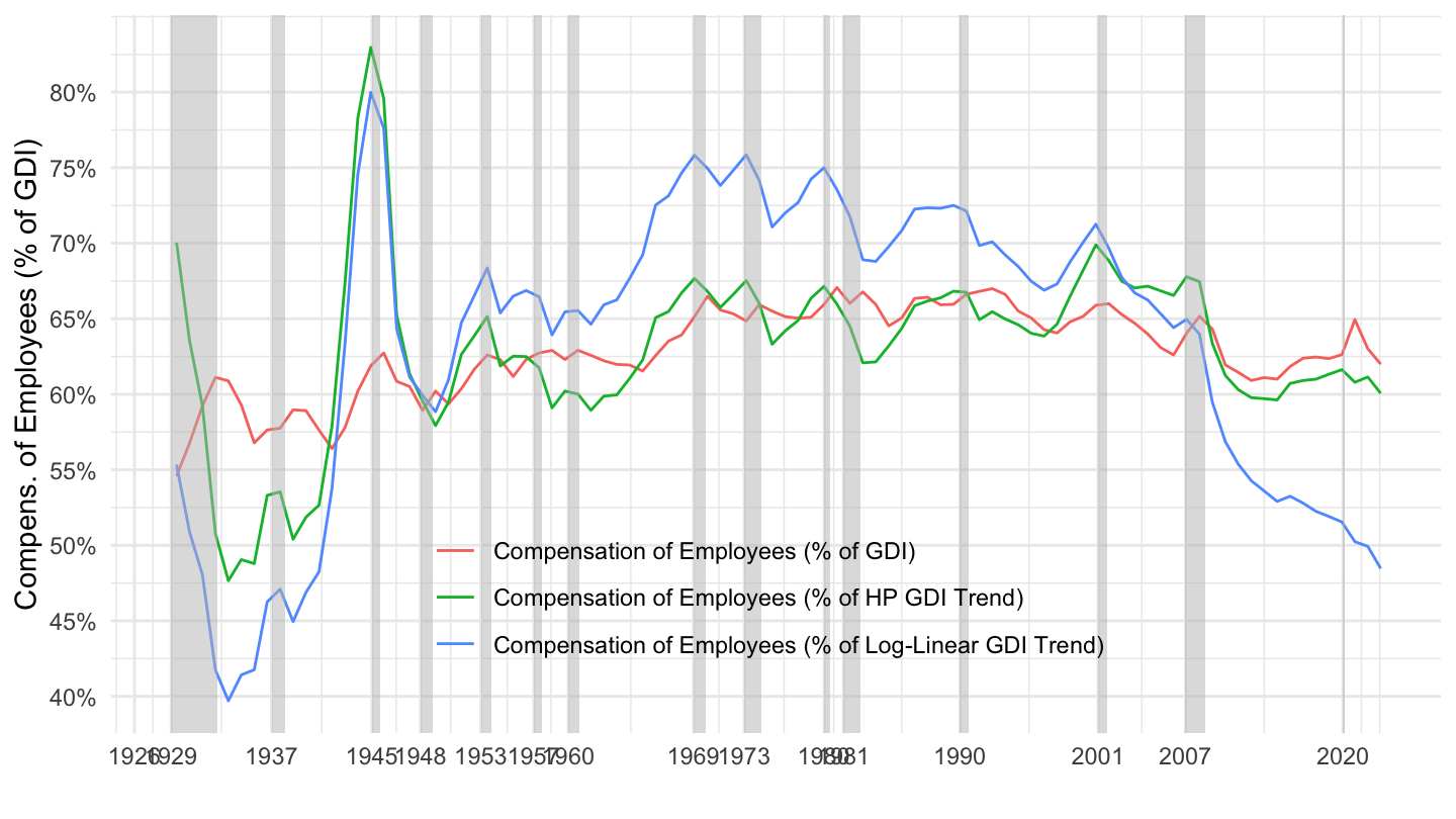

Figure 1: Compensation of Employees.