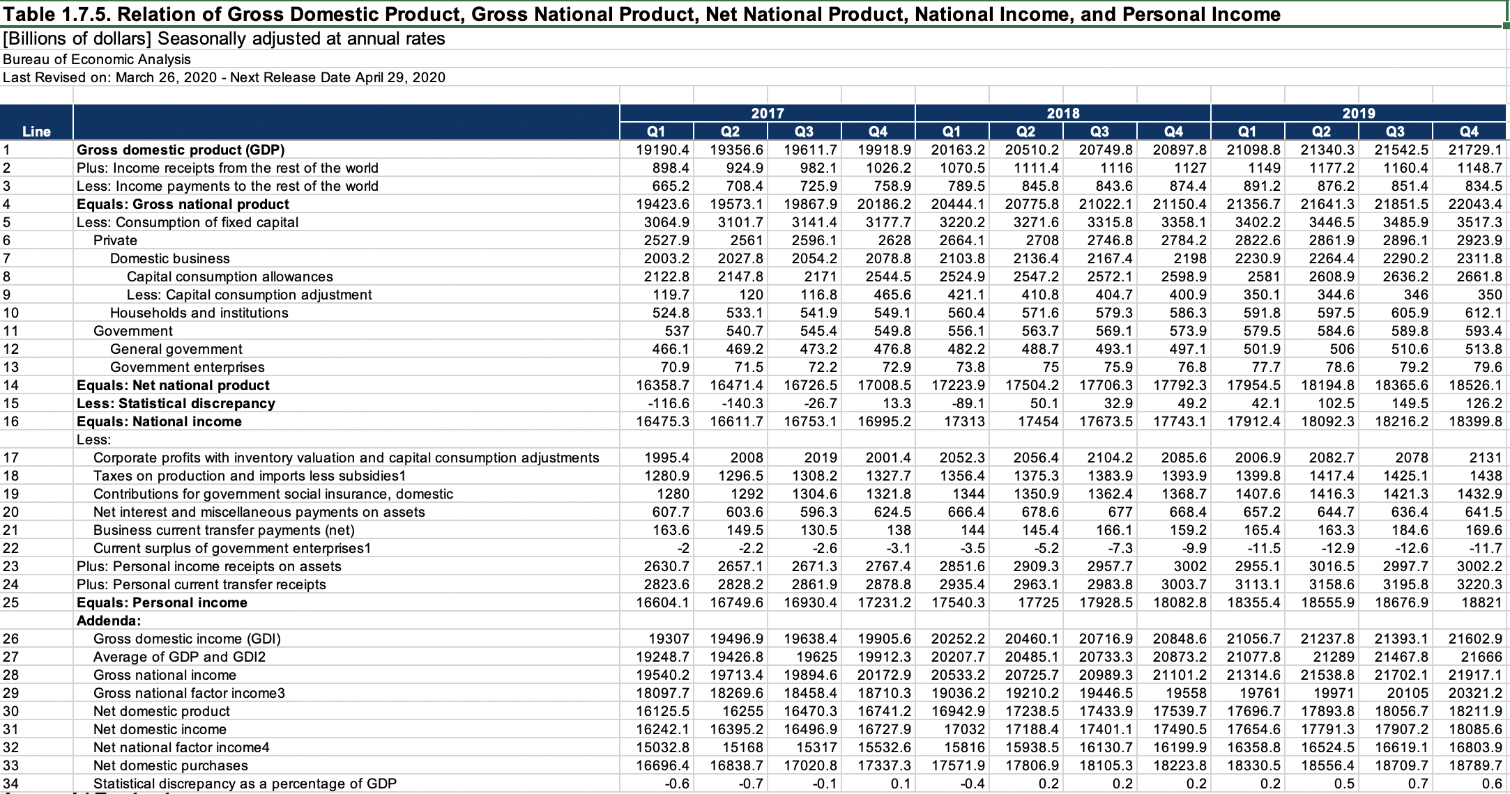
Table 1.7.5. Relation of Gross Domestic Product, Gross National Product, Net National Product, National Income, and Personal Income (A) (Q) - T10705

Data - BEA

~/data/bea/NIPA.html

Info

source	dataset	.html	.RData
bea	T10705	2024-01-06	2023-12-17
bea	T50100	2024-01-06	2023-12-17

Data on US macro

source	dataset	.html	.RData
fred	gdp	2024-02-03	2024-02-11
fred	unr	2024-02-03	2024-02-03
oecd	QNA	2024-01-28	2024-02-03
oecd	SNA_TABLE1	2024-01-28	2024-02-03

LAST_COMPILE

LAST_COMPILE
2024-02-11

Last

date	Nobs
2023-09-30	34

Layout

• NIPA Website. html

GDP and Net National Income

T10705 %>% filter(FREQ == "A") %>% select(-FREQ) %>%
  year_to_date %>%
  group_by(date) %>%
  mutate(value = DataValue/DataValue[LineNumber == 1]) %>%
  filter(LineNumber %in% c(14, 25)) %>%
  ggplot(.) + theme_minimal() +
  geom_line(aes(x = date, y = value, color = LineDescription)) +
  theme(legend.title = element_blank(),
        legend.position = c(0.7, 0.9)) +
  geom_rect(data = nber_recessions %>%
              filter(Peak > as.Date("1928-01-01")), 
            aes(xmin = Peak, xmax = Trough, ymin = -Inf, ymax = +Inf), 
            fill = 'grey', alpha = 0.5) + 
  scale_x_date(breaks = seq(1930, 2100, 5) %>% paste0("-01-01") %>% as.Date,
               labels = date_format("%Y")) +
  ylab("% of GDP") + xlab("") +
  
  scale_y_continuous(breaks = 0.01*seq(0, 100, 2),
                     labels = scales::percent_format(accuracy = 1))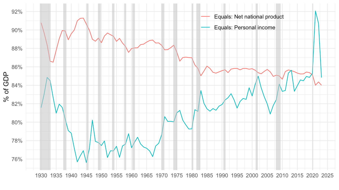

Taxes on Production and Corporate profits

T10705 %>% filter(FREQ == "A") %>% select(-FREQ) %>%
  year_to_date %>%
  group_by(date) %>%
  mutate(value = DataValue/DataValue[LineNumber == 1]) %>%
  filter(LineNumber %in% c(17, 18, 23)) %>%
  ggplot(.) + theme_minimal() +
  geom_line(aes(x = date, y = value, color = LineDescription)) +
  theme(legend.title = element_blank(),
        legend.position = c(0.6, 0.2)) +
  geom_rect(data = nber_recessions %>%
              filter(Peak > as.Date("1928-01-01")), 
            aes(xmin = Peak, xmax = Trough, ymin = -Inf, ymax = +Inf), 
            fill = 'grey', alpha = 0.5) + 
  scale_x_date(breaks = seq(1930, 2100, 5) %>% paste0("-01-01") %>% as.Date,
               labels = date_format("%Y")) +
  ylab("% of GDP") + xlab("") +
  
  scale_y_continuous(breaks = 0.01*seq(0, 100, 2),
                     labels = scales::percent_format(accuracy = 1))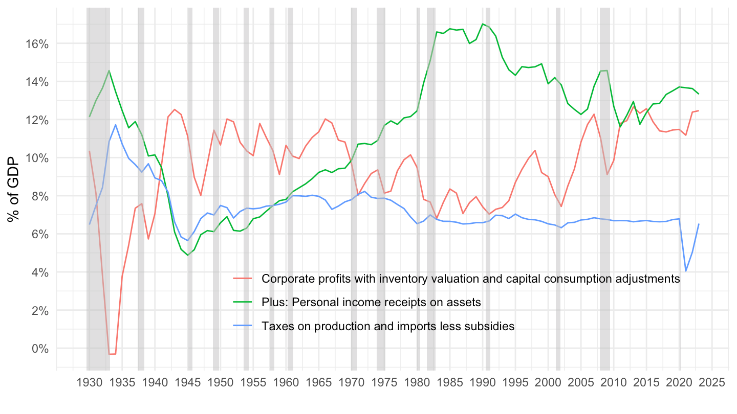

Compare profits and asset transfers

T10705 %>% filter(FREQ == "A") %>% select(-FREQ) %>%
  year_to_date %>%
  group_by(date) %>%
  mutate(value = DataValue/DataValue[LineNumber == 1]) %>%
  filter(LineNumber %in% c(5, 25)) %>%
  ggplot(.) + theme_minimal() +
  geom_line(aes(x = date, y = value, color = LineDescription)) +
  theme(legend.title = element_blank(),
        legend.position = c(0.6, 0.2)) +
  geom_rect(data = nber_recessions %>%
              filter(Peak > as.Date("1928-01-01")), 
            aes(xmin = Peak, xmax = Trough, ymin = -Inf, ymax = +Inf), 
            fill = 'grey', alpha = 0.5) + 
  scale_x_date(breaks = seq(1930, 2100, 5) %>% paste0("-01-01") %>% as.Date,
               labels = date_format("%Y")) +
  ylab("% of Personal Income") + xlab("") +
  
  scale_y_continuous(breaks = 0.01*seq(0, 100, 10),
                     labels = scales::percent_format(accuracy = 1))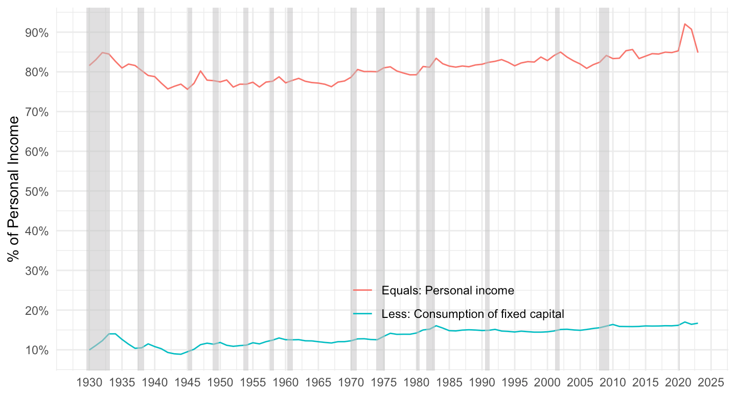

Consumption fixed capital

T10705 %>% filter(FREQ == "A") %>% select(-FREQ) %>%
  year_to_date %>%
  group_by(date) %>%
  mutate(value = DataValue/DataValue[LineNumber == 1]) %>%
  filter(LineNumber %in% c(5, 17)) %>%
  ggplot(.) + theme_minimal() +
  geom_line(aes(x = date, y = value, color = LineDescription)) +
  theme(legend.title = element_blank(),
        legend.position = c(0.6, 0.2)) +
  geom_rect(data = nber_recessions %>%
              filter(Peak > as.Date("1928-01-01")), 
            aes(xmin = Peak, xmax = Trough, ymin = -Inf, ymax = +Inf), 
            fill = 'grey', alpha = 0.5) + 
  scale_x_date(breaks = seq(1930, 2100, 5) %>% paste0("-01-01") %>% as.Date,
               labels = date_format("%Y")) +
  ylab("% of Personal Income") + xlab("") +
  
  scale_y_continuous(breaks = 0.01*seq(0, 30, 1),
                     labels = scales::percent_format(accuracy = 1))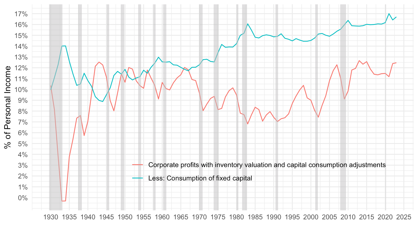

Personal income

T10705 %>% filter(FREQ == "A") %>% select(-FREQ) %>%
  year_to_date %>%
  group_by(date) %>%
  mutate(value = DataValue/DataValue[1]) %>%
  filter(LineNumber %in% c(25, 16)) %>%
  ggplot(.) + theme_minimal() +
  geom_line(aes(x = date, y = value, color = LineDescription)) +
  theme(legend.title = element_blank(),
        legend.position = c(0.6, 0.9)) +
  geom_rect(data = nber_recessions %>%
              filter(Peak > as.Date("1928-01-01")), 
            aes(xmin = Peak, xmax = Trough, ymin = -Inf, ymax = +Inf), 
            fill = 'grey', alpha = 0.5) + 
  ylab("% of GDP") + xlab("") +
  
  scale_y_continuous(breaks = 0.01*seq(0, 100, 2),
                     labels = scales::percent_format(accuracy = 1))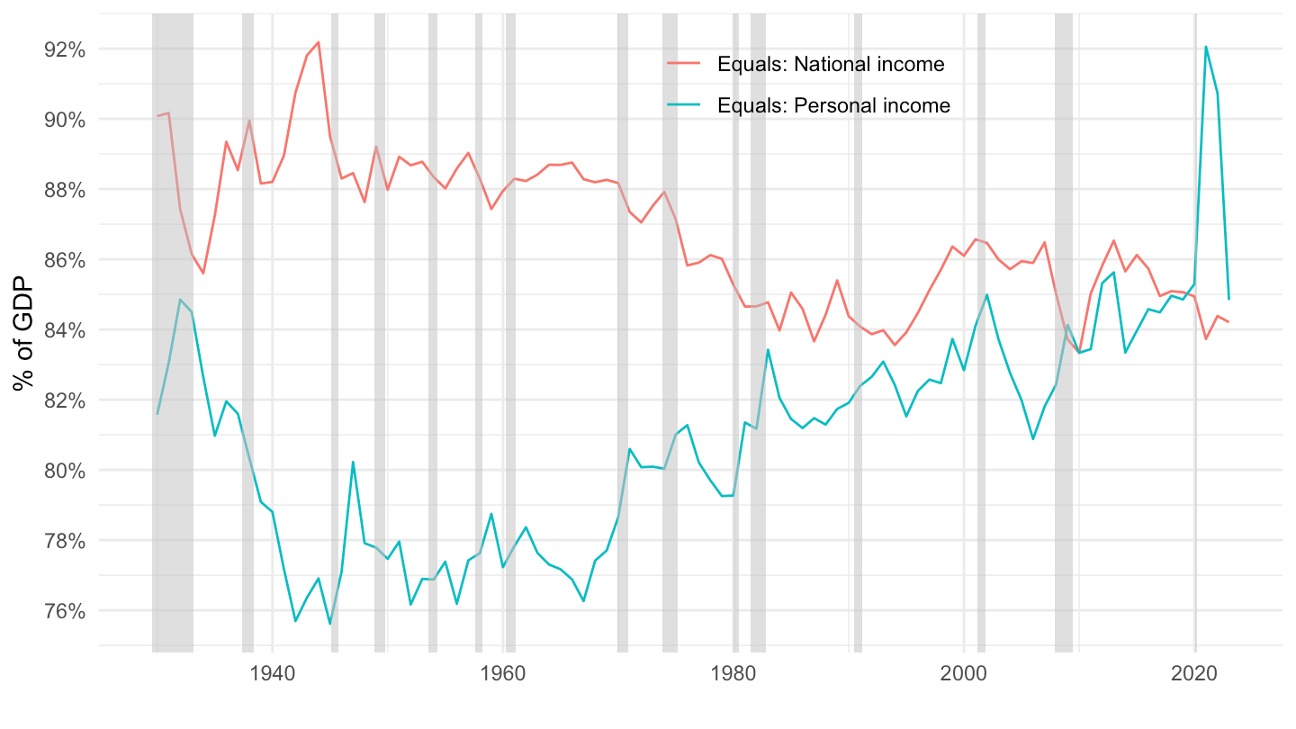

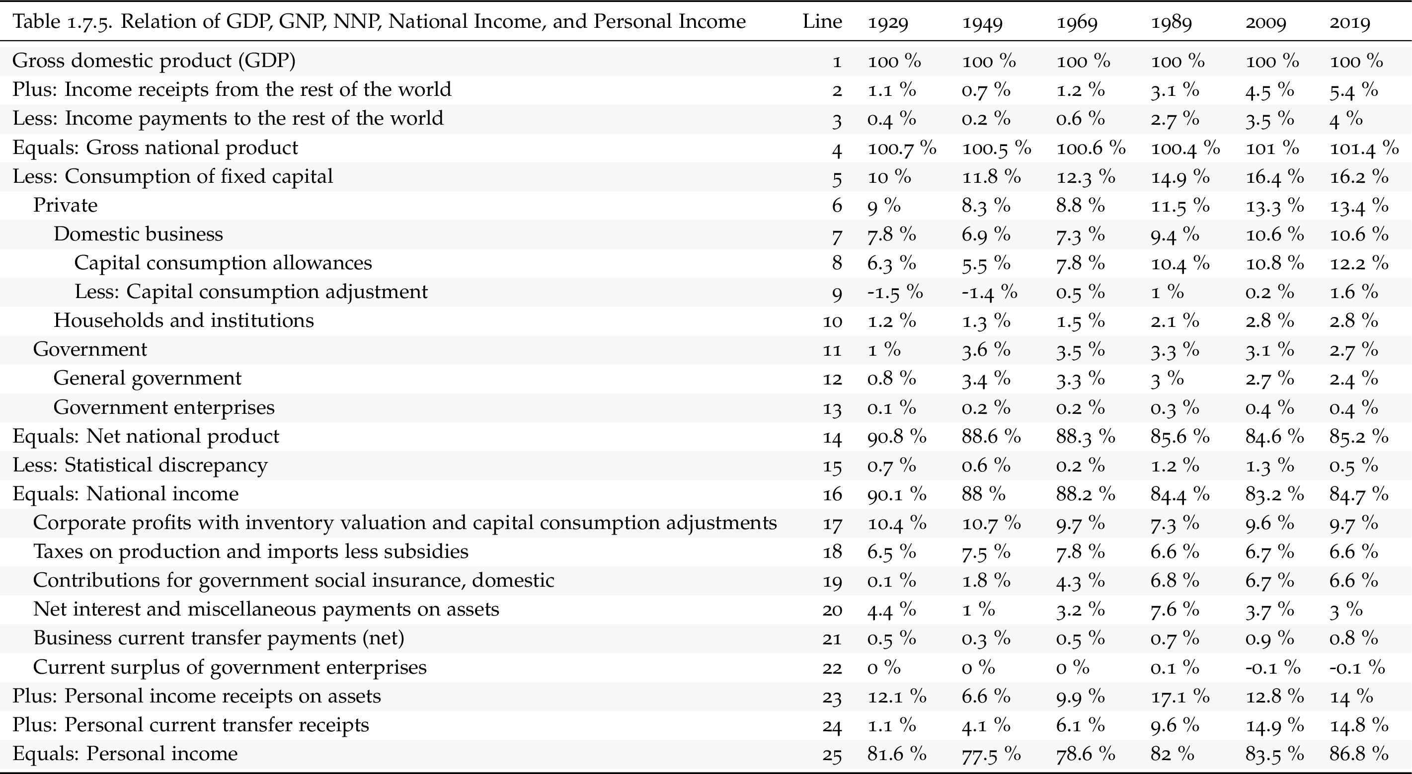
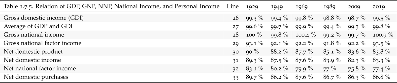
1938, 1958, 1978, 1998, 2018 Table

Percent

T10705 %>% filter(FREQ == "A") %>% select(-FREQ) %>%
  year_to_date %>%
  mutate(year = year(date)) %>%
  filter(year %in% c(1929, 1949, 1969, 1989, 2009, 2019)) %>%
  group_by(year) %>%
  mutate(value = round(100*DataValue/DataValue[1], 1)) %>%
  ungroup %>%
  select(2, 3, 6, 7) %>%
  spread(year, value) %>%
  mutate_at(vars(-1, -2), funs(ifelse(is.na(.), "", paste0(., " %")))) %>%
  select(-LineNumber) %>%
  setNames(c("", names(.)[2:7])) %>%
  knitr::kable(booktabs = TRUE,
               linesep = "") %>%
  kable_styling(bootstrap_options = c("striped", "hover", "condensed"),
                latex_options = c("striped", "hold_position"))

	1929	1949	1969	1989	2009	2019
Gross domestic product (GDP)	100 %	100 %	100 %	100 %	100 %	100 %
Plus: Income receipts from the rest of the world	1.1 %	0.7 %	1.2 %	3.1 %	4.8 %	5.5 %
Less: Income payments to the rest of the world	0.4 %	0.2 %	0.6 %	2.7 %	3.7 %	4.1 %
Equals: Gross national product	100.7 %	100.5 %	100.6 %	100.4 %	101 %	101.3 %
Less: Consumption of fixed capital	10 %	11.8 %	12.3 %	14.9 %	16.4 %	16.2 %
Private	9 %	8.3 %	8.8 %	11.5 %	13.3 %	13.4 %
Domestic business	7.8 %	6.9 %	7.3 %	9.4 %	10.6 %	10.5 %
Capital consumption allowances	6.3 %	5.5 %	7.8 %	10.4 %	10.8 %	12.6 %
Less: Capital consumption adjustment	-1.5 %	-1.4 %	0.5 %	1 %	0.2 %	2 %
Households and institutions	1.2 %	1.3 %	1.5 %	2.1 %	2.7 %	2.9 %
Government	1 %	3.6 %	3.5 %	3.3 %	3.1 %	2.8 %
General government	0.8 %	3.4 %	3.3 %	3 %	2.7 %	2.4 %
Government enterprises	0.1 %	0.2 %	0.2 %	0.3 %	0.4 %	0.4 %
Equals: Net national product	90.8 %	88.6 %	88.3 %	85.6 %	84.7 %	85.1 %
Less: Statistical discrepancy	0.7 %	0.6 %	0.2 %	1.2 %	1.3 %	0.2 %
Equals: National income	90.1 %	88 %	88.2 %	84.4 %	83.3 %	84.9 %
Corporate profits with inventory valuation and capital consumption adjustments	10.4 %	10.7 %	9.7 %	7.4 %	9.8 %	11.5 %
Taxes on production and imports less subsidies	6.5 %	7.5 %	7.8 %	6.6 %	6.7 %	6.8 %
Contributions for government social insurance, domestic	0.1 %	1.8 %	4.3 %	6.8 %	6.7 %	6.6 %
Net interest and miscellaneous payments on assets	4.4 %	1 %	3.2 %	7.5 %	3.6 %	2.4 %
Business current transfer payments (net)	0.5 %	0.3 %	0.5 %	0.7 %	0.9 %	0.7 %
Current surplus of government enterprises	0 %	0 %	0 %	0.1 %	-0.1 %	-0.1 %
Plus: Personal income receipts on assets	12.1 %	6.6 %	9.9 %	17 %	12.7 %	13.7 %
Plus: Personal current transfer receipts	1.1 %	4.1 %	6.1 %	9.6 %	14.8 %	14.6 %
Equals: Personal income	81.6 %	77.5 %	78.6 %	81.9 %	83.3 %	85.3 %
Gross domestic income (GDI)	99.3 %	99.4 %	99.8 %	98.8 %	98.7 %	99.8 %
Average of GDP and GDI	99.6 %	99.7 %	99.9 %	99.4 %	99.3 %	99.9 %
Gross national income	100 %	99.8 %	100.4 %	99.2 %	99.7 %	101.1 %
Gross national factor income	93.1 %	92.1 %	92.2 %	91.8 %	92.3 %	93.6 %
Net domestic product	90 %	88.2 %	87.7 %	85.1 %	83.6 %	83.8 %
Net domestic income	89.3 %	87.5 %	87.6 %	83.9 %	82.3 %	83.6 %
Net national factor income	83.1 %	80.2 %	79.9 %	77 %	75.9 %	77.5 %
Net domestic purchases	89.7 %	86.2 %	87.6 %	86.7 %	86.5 %	86.5 %
Statistical discrepancy as a percentage of GDP	0 %	0 %	0 %	0 %	0 %	0 %

Percent

T10705 %>% filter(FREQ == "A") %>% select(-FREQ) %>%
  year_to_date %>%
  mutate(year = year(date)) %>%
  filter(year %in% c(1938, 1958, 1978, 1998, 2018)) %>%
  group_by(year) %>%
  mutate(value = round(100*DataValue/DataValue[1], 1)) %>%
  ungroup %>%
  select(2, 3, 6, 7) %>%
  spread(year, value) %>%
  {if (is_html_output()) datatable(., filter = 'top', rownames = F) else .}

Percent - pdf

Billions

T10705 %>% filter(FREQ == "A") %>% select(-FREQ) %>%
  year_to_date %>%
  mutate(year = year(date)) %>%
  filter(year %in% c(1938, 1958, 1978, 1998, 2018)) %>%
  group_by(year) %>%
  mutate(value = round(DataValue/1000)) %>%
  ungroup %>%
  select(2, 3, 6, 7) %>%
  spread(year, value) %>%
  {if (is_html_output()) datatable(., filter = 'top', rownames = F) else .}