Social Expenditure - Aggregated data - SOCX_AGG
Data - OECD
Info
Data on germany
| source | dataset | Title | .html | .rData |
|---|---|---|---|---|
| oecd | QNA | Quarterly National Accounts | 2026-07-24 | 2026-07-24 |
| wdi | NY.GDP.PCAP.PP.CD | GDP per capita, PPP (current international D) | 2026-07-25 | 2026-07-24 |
LAST_COMPILE
| LAST_COMPILE |
|---|
| 2026-07-26 |
Last
| obsTime | Nobs |
|---|---|
| 2022 | 27 |
Number of Observations
Code
SOCX_AGG %>%
  left_join(SOCX_AGG_var$BRANCH, by = "BRANCH") %>%
  left_join(SOCX_AGG_var$TYPEXP, by = "TYPEXP") %>%
  group_by(BRANCH, Branch, TYPEXP, Typexp, SOURCE, TYPROG, UNIT) %>%
  summarise(Nobs = n()) %>%
  arrange(-Nobs) %>%
  {if (is_html_output()) datatable(., filter = 'top', rownames = F) else .}
SOURCE
Code
SOCX_AGG %>%
  left_join(SOCX_AGG_var$SOURCE, by = "SOURCE") %>%
  group_by(SOURCE, Source) %>%
  summarise(Nobs = n()) %>%
  arrange(-Nobs) %>%
{if (is_html_output()) print_table(.) else .}| SOURCE | Source | Nobs |
|---|---|---|
| 10 | Public | 620962 |
| 20 | Mandatory private | 555275 |
| 10_20 | Public and mandatory private | 486610 |
| 20_30 | Private (Mandatory and Voluntary) | 99093 |
| 30 | Voluntary private | 46257 |
| 40 | Net Public | 380 |
| 50 | Net Total | 379 |
BRANCH
Code
SOCX_AGG %>%
  left_join(SOCX_AGG_var$BRANCH, by = "BRANCH") %>%
  group_by(BRANCH, Branch) %>%
  summarise(Nobs = n()) %>%
  arrange(-Nobs) %>%
{if (is_html_output()) print_table(.) else .}| BRANCH | Branch | Nobs |
|---|---|---|
| 3 | Incapacity related | 276495 |
| 5 | Family | 216535 |
| 1 | Old age | 208398 |
| 1_2 | Old age and Survivors | 187863 |
| 6 | Active labour market programmes | 181100 |
| 9 | Other social policy areas | 177418 |
| 2 | Survivors | 165123 |
| 7 | Unemployment | 111688 |
| 8 | Housing | 107355 |
| 90 | Total | 95210 |
| 4 | Health | 81771 |
TYPEXP
Code
SOCX_AGG %>%
  left_join(SOCX_AGG_var$TYPEXP, by = "TYPEXP") %>%
  group_by(TYPEXP, Typexp) %>%
  summarise(Nobs = n()) %>%
  arrange(-Nobs) %>%
{if (is_html_output()) print_table(.) else .}| TYPEXP | Typexp | Nobs |
|---|---|---|
| 1 | Cash benefits | 722474 |
| 2 | Benefits in kind | 584666 |
| 0 | Total | 501816 |
TYPROG
Code
SOCX_AGG %>%
  left_join(SOCX_AGG_var$TYPROG, by = "TYPROG") %>%
  group_by(TYPROG, Typrog) %>%
  summarise(Nobs = n()) %>%
  arrange(-Nobs) %>%
  print_table_conditional()
UNIT
Code
SOCX_AGG %>%
  left_join(SOCX_AGG_var$UNIT, by = "UNIT") %>%
  group_by(UNIT, Unit) %>%
  summarise(Nobs = n()) %>%
  arrange(-Nobs) %>%
print_table_conditional()| UNIT | Unit | Nobs |
|---|---|---|
| NCUR | NA | 326763 |
| PCT_GDP | NA | 320149 |
| PPPVH | NA | 315628 |
| PPPH | NA | 310505 |
| NCST | NA | 309449 |
| PCT_GOV | NA | 226462 |
COUNTRY
Code
SOCX_AGG %>%
  left_join(SOCX_AGG_var$COUNTRY, by = "COUNTRY") %>%
  group_by(COUNTRY, Country) %>%
  summarise(Nobs = n()) %>%
  arrange(-Nobs) %>%
  print_table_conditional()
obsTime
Code
SOCX_AGG %>%
  group_by(obsTime) %>%
  summarise(Nobs = n()) %>%
{if (is_html_output()) datatable(., filter = 'top', rownames = F) else .}All
Cash
Code
SOCX_AGG %>%
  filter(SOURCE == 10,
         TYPROG == 0,
         TYPEXP == 1,
         COUNTRY %in% c("USA", "FRA", "DEU", "GBR"),
         UNIT == "PCT_GDP",
         obsTime == "2015") %>%
  left_join(SOCX_AGG_var$BRANCH, by = "BRANCH") %>%
  select(BRANCH, Branch, COUNTRY, obsValue) %>%
  spread(COUNTRY, obsValue) %>%
  mutate_at(vars(-BRANCH, -Branch), funs(round(., digits = 1))) -> SOC_AGG_TYPEXP_1

do.call(save, list("SOC_AGG_TYPEXP_1", file = "SOC_AGG_TYPEXP_1.RData"))

SOC_AGG_TYPEXP_1 %>%
  {if (is_html_output()) datatable(., filter = 'top', rownames = F) else .}
In-kind
Code
SOCX_AGG %>%
  filter(SOURCE == 10,
         TYPROG == 0,
         TYPEXP == 2,
         COUNTRY %in% c("USA", "FRA", "DEU", "GBR"),
         UNIT == "PCT_GDP",
         obsTime == "2015") %>%
  left_join(SOCX_AGG_var$BRANCH, by = "BRANCH") %>%
  select(BRANCH, Branch, COUNTRY, obsValue) %>%
  spread(COUNTRY, obsValue) %>%
  mutate_at(vars(-BRANCH, -Branch), funs(round(., digits = 1))) -> SOC_AGG_TYPEXP_2

do.call(save, list("SOC_AGG_TYPEXP_2", file = "SOC_AGG_TYPEXP_2.RData"))

SOC_AGG_TYPEXP_2 %>%
  {if (is_html_output()) datatable(., filter = 'top', rownames = F) else .}
Total
Code
SOCX_AGG %>%
  filter(SOURCE == 10,
         TYPROG == 0,
         TYPEXP == 0,
         COUNTRY %in% c("USA", "FRA", "DEU", "GBR"),
         UNIT == "PCT_GDP",
         obsTime == "2015") %>%
  left_join(SOCX_AGG_var$BRANCH, by = "BRANCH") %>%
  select(BRANCH, Branch, COUNTRY, obsValue) %>%
  spread(COUNTRY, obsValue) %>%
  mutate_at(vars(-BRANCH, -Branch), funs(round(., digits = 1))) -> SOC_AGG_TYPEXP_0

do.call(save, list("SOC_AGG_TYPEXP_0", file = "SOC_AGG_TYPEXP_0.RData"))

SOC_AGG_TYPEXP_0 %>%
  {if (is_html_output()) datatable(., filter = 'top', rownames = F) else .}
Total - Cash benefits (Branch 90)
World
Code
SOCX_AGG %>%
  filter(SOURCE == 10,
         TYPROG == 0,
         TYPEXP == 1,
         BRANCH == 90,
         UNIT == "PCT_GDP") %>%
  left_join(SOCX_AGG_var$COUNTRY, by = "COUNTRY") %>%
  year_to_enddate %>%
  mutate(year = year(date)) %>%
  filter(year %in% c(1990, 2000, 2015)) %>%
  arrange(Country, year) %>%
  group_by(Country) %>%
  summarise(`1990 (% GDP)` = obsValue[1],
            `2000 (% GDP)` = obsValue[2],
            `2015 (% GDP)` = obsValue[3],
            `Delta 2000-15` = obsValue[3] - obsValue[2]) %>%
  arrange(-`2015 (% GDP)`) %>%
  mutate_at(vars(-Country), funs(round(., digits = 1))) -> SOC_AGG_BRANCH_90

# do.call(save, list("SOC_AGG_BRANCH_90", file = "SOC_AGG_BRANCH_90.RData"))

SOC_AGG_BRANCH_90 %>%
  {if (is_html_output()) datatable(., filter = 'top', rownames = F) else .}
United States, United Kingdom, Australia
Code
SOCX_AGG %>%
  filter(SOURCE == 10,
         TYPROG == 0,
         TYPEXP == 1,
         BRANCH == 90,
         UNIT == "PCT_GDP",
         COUNTRY %in% c("USA", "GBR", "AUS")) %>%
  left_join(SOCX_AGG_var$COUNTRY, by = "COUNTRY") %>%
  year_to_date %>%
  rename(Location = Country) %>%
  left_join(colors, by = c("Location" = "country")) %>%
  mutate(obsValue = obsValue / 100) %>%
  ggplot() + theme_minimal() + ylab("Total - Cash Benefits (% of GDP)") + xlab("") +
  geom_line(aes(x = date, y = obsValue, color = color)) +
  scale_color_identity() + add_3flags +
  scale_x_date(breaks = seq(1920, 2100, 5) %>% paste0("-01-01") %>% as.Date,
               labels = date_format("%Y")) +
  theme(legend.position = c(0.8, 0.15),
        legend.title = element_blank()) +
  scale_y_continuous(breaks = 0.01*seq(-7, 30, 1),
                     labels = scales::percent_format(accuracy = 1))
France, Germany, Netherlands
Code
SOCX_AGG %>%
  filter(SOURCE == 10,
         TYPROG == 0,
         TYPEXP == 1,
         BRANCH == 90,
         UNIT == "PCT_GDP",
         COUNTRY %in% c("FRA", "DEU", "NLD")) %>%
  left_join(SOCX_AGG_var$COUNTRY, by = "COUNTRY") %>%
  year_to_date %>%
  rename(Location = Country) %>%
  left_join(colors, by = c("Location" = "country")) %>%
  mutate(obsValue = obsValue / 100) %>%
  ggplot() + theme_minimal() + ylab("Total - Cash Benefits (% of GDP)") + xlab("") +
  geom_line(aes(x = date, y = obsValue, color = color)) +
  scale_color_identity() + add_3flags +
  scale_x_date(breaks = seq(1920, 2100, 5) %>% paste0("-01-01") %>% as.Date,
               labels = date_format("%Y")) +
  theme(legend.position = c(0.2, 0.15),
        legend.title = element_blank()) +
  scale_y_continuous(breaks = 0.01*seq(-7, 30, 1),
                     labels = scales::percent_format(accuracy = 1))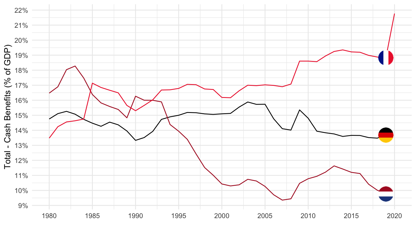
Chile, Denmark, Sweden
Code
SOCX_AGG %>%
  filter(SOURCE == 10,
         TYPROG == 0,
         TYPEXP == 1,
         BRANCH == 90,
         UNIT == "PCT_GDP",
         COUNTRY %in% c("DNK", "SWE", "CHL")) %>%
  left_join(SOCX_AGG_var$COUNTRY, by = "COUNTRY") %>%
  year_to_date %>%
  rename(Location = Country) %>%
  left_join(colors, by = c("Location" = "country")) %>%
  mutate(obsValue = obsValue / 100) %>%
  ggplot() + theme_minimal() + ylab("Total - Cash Benefits (% of GDP)") + xlab("") +
  geom_line(aes(x = date, y = obsValue, color = color)) +
  scale_color_identity() + add_3flags +
  scale_x_date(breaks = seq(1920, 2100, 5) %>% paste0("-01-01") %>% as.Date,
               labels = date_format("%Y")) +
  theme(legend.position = c(0.7, 0.85),
        legend.title = element_blank(),
        legend.direction = "horizontal") +
  scale_y_continuous(breaks = 0.01*seq(-7, 30, 1),
                     labels = scales::percent_format(accuracy = 1))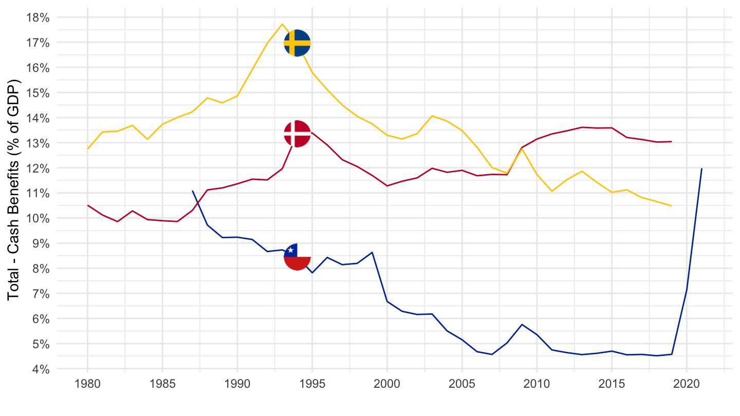
Switzerland, Canada, Sloveinia
Code
SOCX_AGG %>%
  filter(SOURCE == 10,
         TYPROG == 0,
         TYPEXP == 1,
         BRANCH == 90,
         UNIT == "PCT_GDP",
         COUNTRY %in% c("CHE", "CAN", "SVN")) %>%
  left_join(SOCX_AGG_var$COUNTRY, by = "COUNTRY") %>%
  year_to_date %>%
  rename(Location = Country) %>%
  left_join(colors, by = c("Location" = "country")) %>%
  mutate(obsValue = obsValue / 100) %>%
  ggplot() + theme_minimal() + ylab("Total - Cash Benefits (% of GDP)") + xlab("") +
  geom_line(aes(x = date, y = obsValue, color = color)) +
  scale_color_identity() + add_3flags +
  scale_x_date(breaks = seq(1920, 2100, 5) %>% paste0("-01-01") %>% as.Date,
               labels = date_format("%Y")) +
  theme(legend.position = c(0.8, 0.25),
        legend.title = element_blank()) +
  scale_y_continuous(breaks = 0.01*seq(-7, 30, 1),
                     labels = scales::percent_format(accuracy = 1))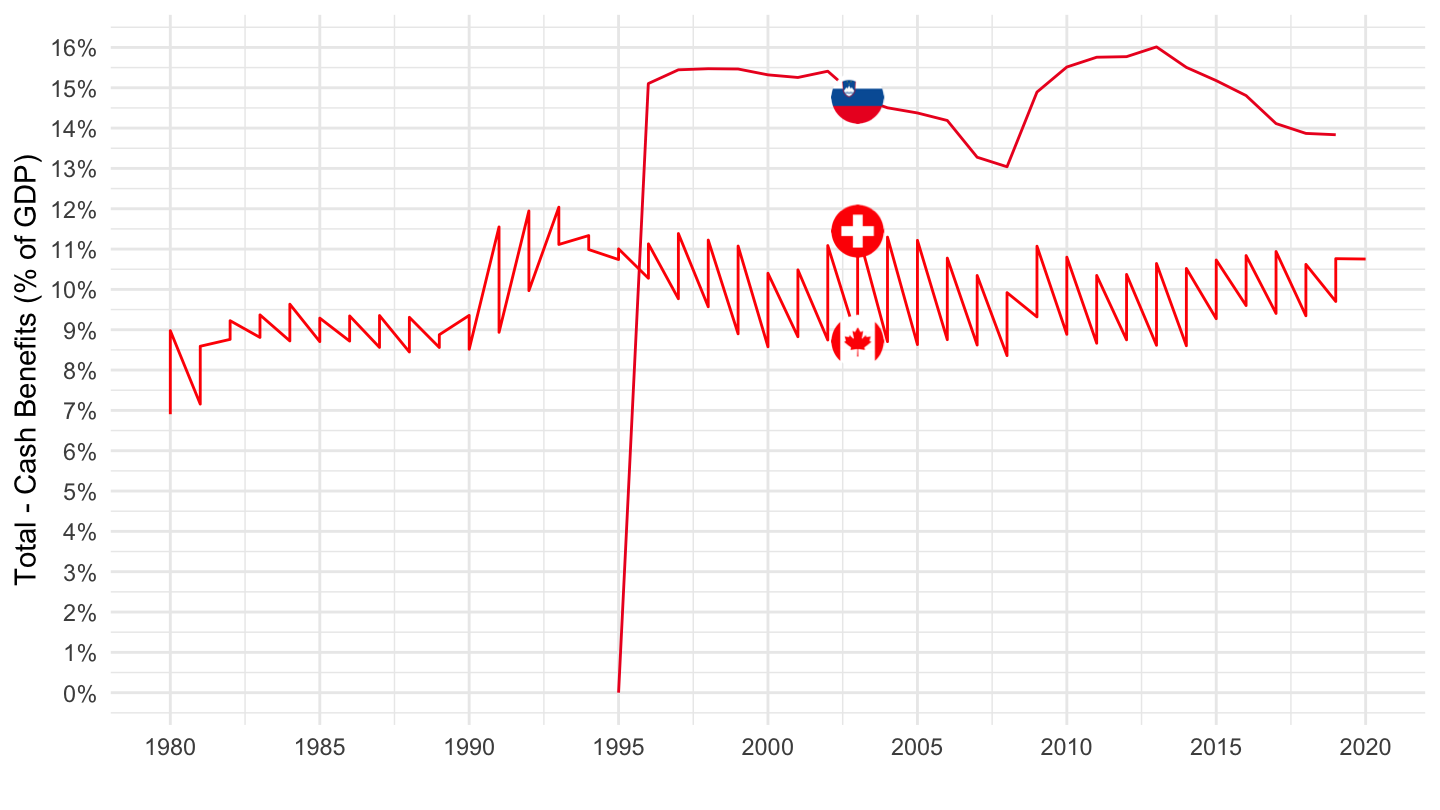
Austria, Belgium, Italy
Code
SOCX_AGG %>%
  filter(SOURCE == 10,
         TYPROG == 0,
         TYPEXP == 1,
         BRANCH == 90,
         UNIT == "PCT_GDP",
         COUNTRY %in% c("BEL", "AUT", "ITA")) %>%
  left_join(SOCX_AGG_var$COUNTRY, by = "COUNTRY") %>%
  year_to_date %>%
  rename(Location = Country) %>%
  left_join(colors, by = c("Location" = "country")) %>%
  mutate(obsValue = obsValue / 100) %>%
  ggplot() + theme_minimal() + ylab("Total - Cash Benefits (% of GDP)") + xlab("") +
  geom_line(aes(x = date, y = obsValue, color = color)) +
  scale_color_identity() + add_3flags +
  scale_x_date(breaks = seq(1920, 2100, 5) %>% paste0("-01-01") %>% as.Date,
               labels = date_format("%Y")) +
  theme(legend.position = c(0.8, 0.25),
        legend.title = element_blank()) +
  scale_y_continuous(breaks = 0.01*seq(-7, 30, 1),
                     labels = scales::percent_format(accuracy = 1))
Old age - Cash benefits (Branch 1)
World
Code
SOCX_AGG %>%
  filter(SOURCE == 10,
         TYPROG == 0,
         TYPEXP == 1,
         BRANCH == 1,
         UNIT == "PCT_GDP") %>%
  left_join(SOCX_AGG_var$COUNTRY, by = "COUNTRY") %>%
  year_to_enddate %>%
  mutate(year = year(date)) %>%
  filter(year %in% c(1990, 2000, 2015)) %>%
  arrange(Country, year) %>%
  group_by(Country, COUNTRY) %>%
  summarise(`1990 (% GDP)` = obsValue[1],
            `2000 (% GDP)` = obsValue[2],
            `2015 (% GDP)` = obsValue[3],
            `Delta 2000-15` = obsValue[3] - obsValue[2]) %>%
  arrange(-`2015 (% GDP)`) %>%
  mutate_at(vars(-Country, -COUNTRY), funs(round(., digits = 1))) %>%
  rename(`Country Name` = Country,
         `Country Code` = COUNTRY) -> SOC_AGG_BRANCH_1

do.call(save, list("SOC_AGG_BRANCH_1", file = "SOC_AGG_BRANCH_1.RData"))

SOC_AGG_BRANCH_1 %>%
  {if (is_html_output()) datatable(., filter = 'top', rownames = F) else .}
Retirement
2015
Code
SOCX_AGG %>%
  filter(TYPROG == 0,
         TYPEXP == 1,
         BRANCH == 1,
         UNIT == "PCT_GDP",
         obsTime == "2014") %>%
  left_join(SOCX_AGG_var$COUNTRY, by = "COUNTRY") %>%
  left_join(SOCX_AGG_var$SOURCE, by = "SOURCE") %>%
  select(Source, COUNTRY, Country, obsValue) %>%
  spread(Source, obsValue) %>%
  arrange(-`Public`) %>%
  {if (is_html_output()) datatable(., filter = 'top', rownames = F) else .}
2017
Code
SOCX_AGG %>%
  filter(TYPROG == 0,
         TYPEXP == 1,
         BRANCH == 1,
         UNIT == "PCT_GDP",
         obsTime == "2017") %>%
  left_join(SOCX_AGG_var$COUNTRY, by = "COUNTRY") %>%
  left_join(SOCX_AGG_var$SOURCE, by = "SOURCE") %>%
  select(Source, COUNTRY, Country, obsValue) %>%
  spread(Source, obsValue) %>%
  arrange(-`Public`) %>%
  {if (is_html_output()) datatable(., filter = 'top', rownames = F) else .}
United States, United Kingdom, Australia
Code
SOCX_AGG %>%
  filter(SOURCE == 10,
         TYPROG == 0,
         TYPEXP == 1,
         BRANCH == 1,
         UNIT == "PCT_GDP",
         COUNTRY %in% c("USA", "GBR", "AUS")) %>%
  left_join(SOCX_AGG_var$COUNTRY, by = "COUNTRY") %>%
  year_to_date %>%
  rename(Location = Country) %>%
  left_join(colors, by = c("Location" = "country")) %>%
  mutate(obsValue = obsValue / 100) %>%
  ggplot() + theme_minimal() + ylab("Old age - Cash Benefits (% of GDP)") + xlab("") +
  geom_line(aes(x = date, y = obsValue, color = color)) +
  scale_color_identity() + add_3flags +
  scale_x_date(breaks = seq(1920, 2100, 5) %>% paste0("-01-01") %>% as.Date,
               labels = date_format("%Y")) +
  theme(legend.position = c(0.35, 0.9),
        legend.title = element_blank(),
        legend.direction = "horizontal") +
  scale_y_continuous(breaks = 0.01*seq(-7, 16, 0.5),
                     labels = scales::percent_format(accuracy = 0.1))
France, Germany, Netherlands
English
Code
SOCX_AGG %>%
  filter(SOURCE == 10,
         TYPROG == 0,
         TYPEXP == 1,
         BRANCH == 1,
         UNIT == "PCT_GDP",
         COUNTRY %in% c("FRA", "DEU", "NLD")) %>%
  left_join(SOCX_AGG_var$COUNTRY, by = "COUNTRY") %>%
  year_to_date %>%
  rename(Location = Country) %>%
  left_join(colors, by = c("Location" = "country")) %>%
  mutate(obsValue = obsValue / 100) %>%
  ggplot() + theme_minimal() + ylab("Old age - Cash Benefits (% of GDP)") + xlab("") +
  geom_line(aes(x = date, y = obsValue, color = color)) +
  scale_color_identity() + add_3flags +
  scale_x_date(breaks = seq(1920, 2100, 5) %>% paste0("-01-01") %>% as.Date,
               labels = date_format("%Y")) +
  theme(legend.position = c(0.25, 0.9),
        legend.title = element_blank(),
        legend.direction = "horizontal") +
  scale_y_continuous(breaks = 0.01*seq(-7, 16, 1),
                     labels = scales::percent_format(accuracy = 0.1))
French
Code
SOCX_AGG %>%
  filter(SOURCE == 10,
         TYPROG == 0,
         TYPEXP == 1,
         BRANCH == 1,
         UNIT == "PCT_GDP",
         COUNTRY %in% c("FRA", "DEU", "NLD")) %>%
  mutate(Country = case_when(COUNTRY == "FRA" ~ "France",
                             COUNTRY == "DEU" ~ "Allemagne",
                             COUNTRY == "NLD" ~ "Pays-Bas")) %>%
  year_to_enddate %>%
  ggplot() + theme_minimal() + ylab("Retraites - Dépenses Monétaires (% of PIB)") + xlab("") +
  geom_line(aes(x = date, y = obsValue / 100, color = Country, linetype = Country)) +
  scale_color_manual(values = viridis(4)[1:3]) +
  scale_x_date(breaks = seq(1920, 2100, 2) %>% paste0("-01-01") %>% as.Date,
               labels = date_format("%Y")) +
  theme(legend.position = c(0.25, 0.9),
        legend.title = element_blank(),
        legend.direction = "horizontal") +
  scale_y_continuous(breaks = 0.01*seq(-7, 16, 1),
                     labels = scales::percent_format(accuracy = 1))
Chile, Denmark, Sweden
Code
SOCX_AGG %>%
  filter(SOURCE == 10,
         TYPROG == 0,
         TYPEXP == 1,
         BRANCH == 1,
         UNIT == "PCT_GDP",
         COUNTRY %in% c("DNK", "SWE", "CHL")) %>%
  left_join(SOCX_AGG_var$COUNTRY, by = "COUNTRY") %>%
  year_to_date %>%
  rename(Location = Country) %>%
  left_join(colors, by = c("Location" = "country")) %>%
  mutate(obsValue = obsValue / 100) %>%
  ggplot() + theme_minimal() + ylab("Old age - Cash Benefits (% of GDP)") + xlab("") +
  geom_line(aes(x = date, y = obsValue, color = color)) +
  scale_color_identity() + add_3flags +
  scale_x_date(breaks = seq(1920, 2100, 5) %>% paste0("-01-01") %>% as.Date,
               labels = date_format("%Y")) +
  theme(legend.position = c(0.25, 0.2),
        legend.title = element_blank()) +
  scale_y_continuous(breaks = 0.01*seq(-7, 16, 0.5),
                     labels = scales::percent_format(accuracy = 0.1))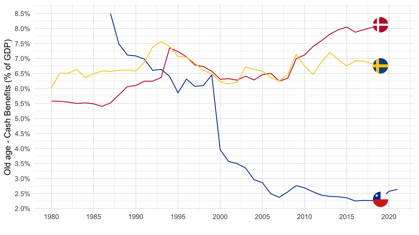
Switzerland, Canada, Sloveinia
Code
SOCX_AGG %>%
  filter(SOURCE == 10,
         TYPROG == 0,
         TYPEXP == 1,
         BRANCH == 1,
         UNIT == "PCT_GDP",
         COUNTRY %in% c("CHE", "CAN", "SVN")) %>%
  left_join(SOCX_AGG_var$COUNTRY, by = "COUNTRY") %>%
  year_to_date %>%
  rename(Location = Country) %>%
  left_join(colors, by = c("Location" = "country")) %>%
  mutate(obsValue = obsValue / 100) %>%
  ggplot() + theme_minimal() + ylab("Old age - Cash Benefits (% of GDP)") + xlab("") +
  geom_line(aes(x = date, y = obsValue, color = color)) +
  scale_color_identity() + add_3flags +
  scale_x_date(breaks = seq(1920, 2100, 5) %>% paste0("-01-01") %>% as.Date,
               labels = date_format("%Y")) +
  theme(legend.position = c(0.15, 0.85),
        legend.title = element_blank()) +
  scale_y_continuous(breaks = 0.01*seq(-7, 16, 1),
                     labels = scales::percent_format(accuracy = 0.1))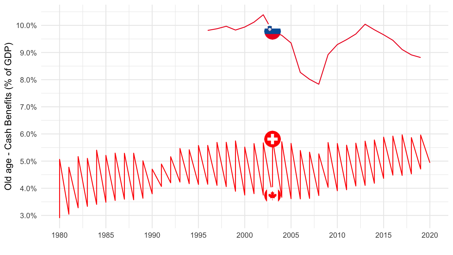
Austria, Belgium, Italy
Code
SOCX_AGG %>%
  filter(SOURCE == 10,
         TYPROG == 0,
         TYPEXP == 1,
         BRANCH == 1,
         UNIT == "PCT_GDP",
         COUNTRY %in% c("BEL", "AUT", "ITA")) %>%
  left_join(SOCX_AGG_var$COUNTRY, by = "COUNTRY") %>%
  year_to_date %>%
  rename(Location = Country) %>%
  left_join(colors, by = c("Location" = "country")) %>%
  mutate(obsValue = obsValue / 100) %>%
  ggplot() + theme_minimal() + ylab("Old age - Cash Benefits (% of GDP)") + xlab("") +
  geom_line(aes(x = date, y = obsValue, color = color)) +
  scale_color_identity() + add_3flags +
  scale_x_date(breaks = seq(1920, 2100, 5) %>% paste0("-01-01") %>% as.Date,
               labels = date_format("%Y")) +
  theme(legend.position = c(0.15, 0.85),
        legend.title = element_blank()) +
  scale_y_continuous(breaks = 0.01*seq(-7, 16, 1),
                     labels = scales::percent_format(accuracy = 0.1))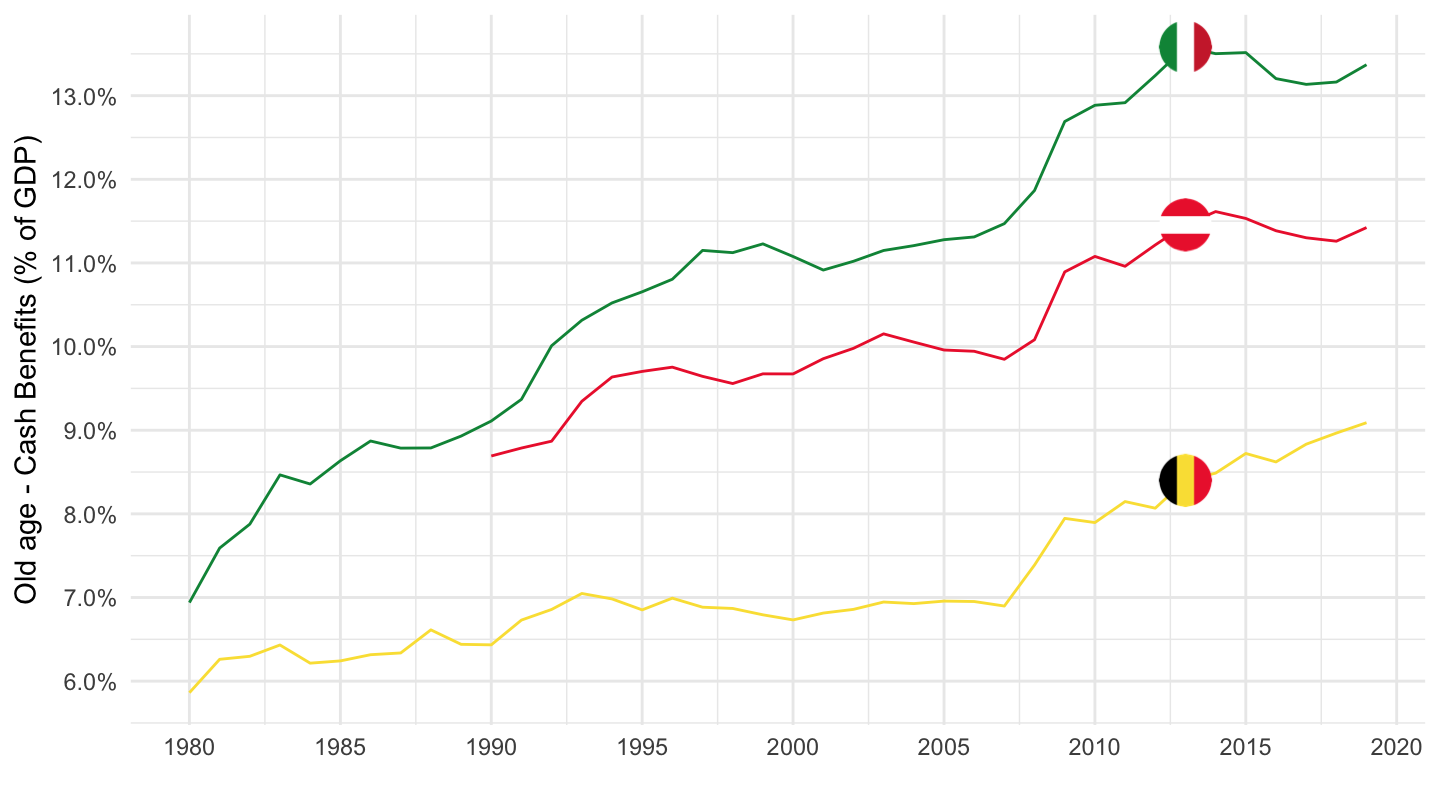
Survivors - Cash benefits (Branch 2)
World
Code
SOCX_AGG %>%
  filter(SOURCE == 10,
         TYPROG == 0,
         TYPEXP == 1,
         BRANCH == 2,
         UNIT == "PCT_GDP") %>%
  left_join(SOCX_AGG_var$COUNTRY, by = "COUNTRY") %>%
  year_to_enddate %>%
  mutate(year = year(date)) %>%
  filter(year %in% c(1990, 2000, 2015)) %>%
  arrange(Country, year) %>%
  group_by(Country, COUNTRY) %>%
  summarise(`1990 (% GDP)` = obsValue[1],
            `2000 (% GDP)` = obsValue[2],
            `2015 (% GDP)` = obsValue[3],
            `Delta 2000-15` = obsValue[3] - obsValue[2]) %>%
  arrange(-`2015 (% GDP)`) %>%
  mutate_at(vars(-Country, -COUNTRY), funs(round(., digits = 1))) %>%
  rename(`Country Name` = Country,
         `Country Code` = COUNTRY) -> SOC_AGG_BRANCH_2

# do.call(save, list("SOC_AGG_BRANCH_2", file = "SOC_AGG_BRANCH_2.RData"))

SOC_AGG_BRANCH_2 %>%
  {if (is_html_output()) datatable(., filter = 'top', rownames = F) else .}
United States, United Kingdom, Australia
Code
SOCX_AGG %>%
  filter(SOURCE == 10,
         TYPROG == 0,
         TYPEXP == 1,
         BRANCH == 2,
         UNIT == "PCT_GDP",
         COUNTRY %in% c("USA", "GBR", "AUS")) %>%
  left_join(SOCX_AGG_var$COUNTRY, by = "COUNTRY") %>%
  year_to_date %>%
  rename(Location = Country) %>%
  left_join(colors, by = c("Location" = "country")) %>%
  mutate(obsValue = obsValue / 100) %>%
  ggplot() + theme_minimal() + ylab("Survivors - Cash Benefits (% of GDP)") + xlab("") +
  geom_line(aes(x = date, y = obsValue, color = color)) +
  scale_color_identity() + add_3flags +
  scale_x_date(breaks = seq(1920, 2100, 5) %>% paste0("-01-01") %>% as.Date,
               labels = date_format("%Y")) +
  theme(legend.position = c(0.65, 0.9),
        legend.title = element_blank(),
        legend.direction = "horizontal") +
  scale_y_continuous(breaks = 0.01*seq(-7, 16, 0.5),
                     labels = scales::percent_format(accuracy = 0.1))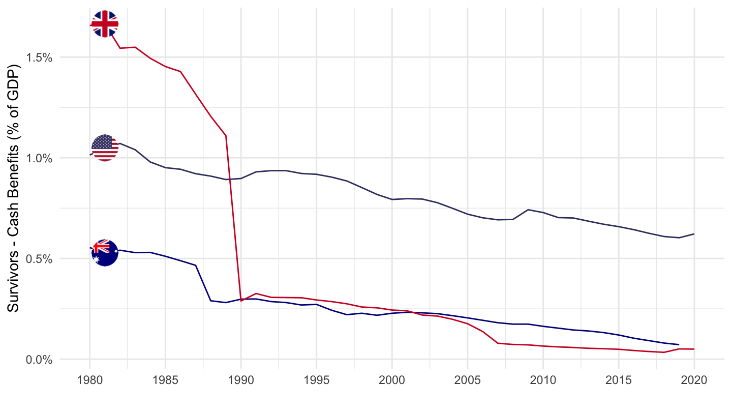
France, Germany, Netherlands
Code
SOCX_AGG %>%
  filter(SOURCE == 10,
         TYPROG == 0,
         TYPEXP == 1,
         BRANCH == 2,
         UNIT == "PCT_GDP",
         COUNTRY %in% c("FRA", "DEU", "NLD")) %>%
  left_join(SOCX_AGG_var$COUNTRY, by = "COUNTRY") %>%
  year_to_date %>%
  rename(Location = Country) %>%
  left_join(colors, by = c("Location" = "country")) %>%
  mutate(obsValue = obsValue / 100) %>%
  ggplot() + theme_minimal() + ylab("Survivors - Cash Benefits (% of GDP)") + xlab("") +
  geom_line(aes(x = date, y = obsValue, color = color)) +
  scale_color_identity() + add_3flags +
  scale_x_date(breaks = seq(1920, 2100, 5) %>% paste0("-01-01") %>% as.Date,
               labels = date_format("%Y")) +
  theme(legend.position = c(0.25, 0.9),
        legend.title = element_blank(),
        legend.direction = "horizontal") +
  scale_y_continuous(breaks = 0.01*seq(-7, 16, 0.5),
                     labels = scales::percent_format(accuracy = 0.1))
Chile, Denmark, Sweden
Code
SOCX_AGG %>%
  filter(SOURCE == 10,
         TYPROG == 0,
         TYPEXP == 1,
         BRANCH == 2,
         UNIT == "PCT_GDP",
         COUNTRY %in% c("DNK", "SWE", "CHL")) %>%
  left_join(SOCX_AGG_var$COUNTRY, by = "COUNTRY") %>%
  year_to_date %>%
  rename(Location = Country) %>%
  left_join(colors, by = c("Location" = "country")) %>%
  mutate(obsValue = obsValue / 100) %>%
  ggplot() + theme_minimal() + ylab("Survivors - Cash Benefits (% of GDP)") + xlab("") +
  geom_line(aes(x = date, y = obsValue, color = color)) +
  scale_color_identity() + add_3flags +
  scale_x_date(breaks = seq(1920, 2100, 5) %>% paste0("-01-01") %>% as.Date,
               labels = date_format("%Y")) +
  theme(legend.position = c(0.25, 0.2),
        legend.title = element_blank()) +
  scale_y_continuous(breaks = 0.01*seq(-7, 16, 0.5),
                     labels = scales::percent_format(accuracy = 0.1))
Switzerland, Canada, Sloveinia
Code
SOCX_AGG %>%
  filter(SOURCE == 10,
         TYPROG == 0,
         TYPEXP == 1,
         BRANCH == 2,
         UNIT == "PCT_GDP",
         COUNTRY %in% c("CHE", "CAN", "SVN")) %>%
  left_join(SOCX_AGG_var$COUNTRY, by = "COUNTRY") %>%
  year_to_date %>%
  rename(Location = Country) %>%
  left_join(colors, by = c("Location" = "country")) %>%
  mutate(obsValue = obsValue / 100) %>%
  ggplot() + theme_minimal() + ylab("Survivors - Cash Benefits (% of GDP)") + xlab("") +
  geom_line(aes(x = date, y = obsValue, color = color)) +
  scale_color_identity() + add_3flags +
  scale_x_date(breaks = seq(1920, 2100, 5) %>% paste0("-01-01") %>% as.Date,
               labels = date_format("%Y")) +
  theme(legend.position = c(0.15, 0.85),
        legend.title = element_blank()) +
  scale_y_continuous(breaks = 0.01*seq(-7, 16, 1),
                     labels = scales::percent_format(accuracy = 0.1))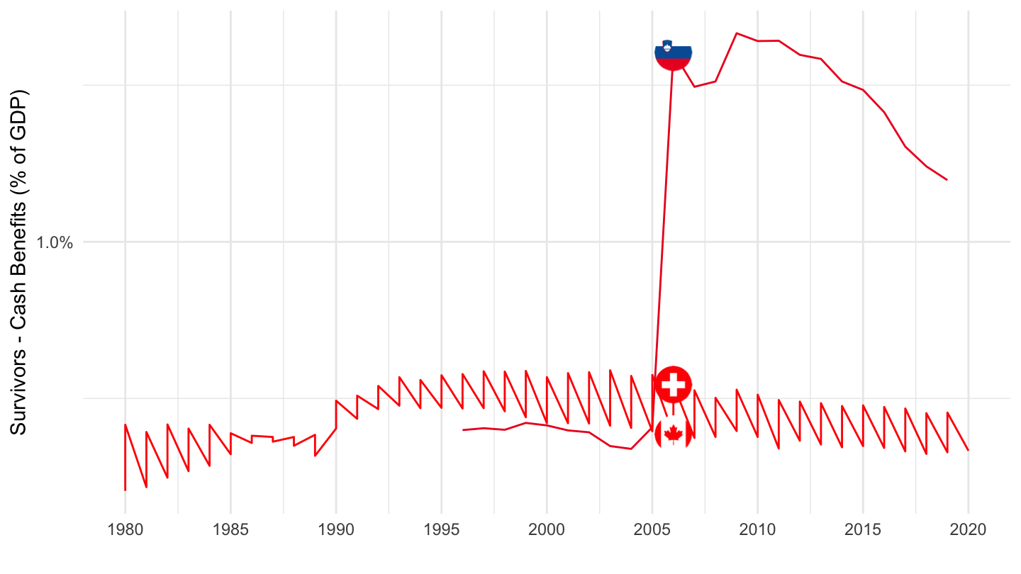
Austria, Belgium, Italy
Code
SOCX_AGG %>%
  filter(SOURCE == 10,
         TYPROG == 0,
         TYPEXP == 1,
         BRANCH == 2,
         UNIT == "PCT_GDP",
         COUNTRY %in% c("BEL", "AUT", "ITA")) %>%
  left_join(SOCX_AGG_var$COUNTRY, by = "COUNTRY") %>%
  year_to_date %>%
  rename(Location = Country) %>%
  left_join(colors, by = c("Location" = "country")) %>%
  mutate(obsValue = obsValue / 100) %>%
  ggplot() + theme_minimal() + ylab("Survivors - Cash Benefits (% of GDP)") + xlab("") +
  geom_line(aes(x = date, y = obsValue, color = color)) +
  scale_color_identity() + add_3flags +
  scale_x_date(breaks = seq(1920, 2100, 5) %>% paste0("-01-01") %>% as.Date,
               labels = date_format("%Y")) +
  theme(legend.position = c(0.35, 0.25),
        legend.title = element_blank(),
        legend.direction = "horizontal") +
  scale_y_continuous(breaks = 0.01*seq(-7, 16, 0.5),
                     labels = scales::percent_format(accuracy = 0.1))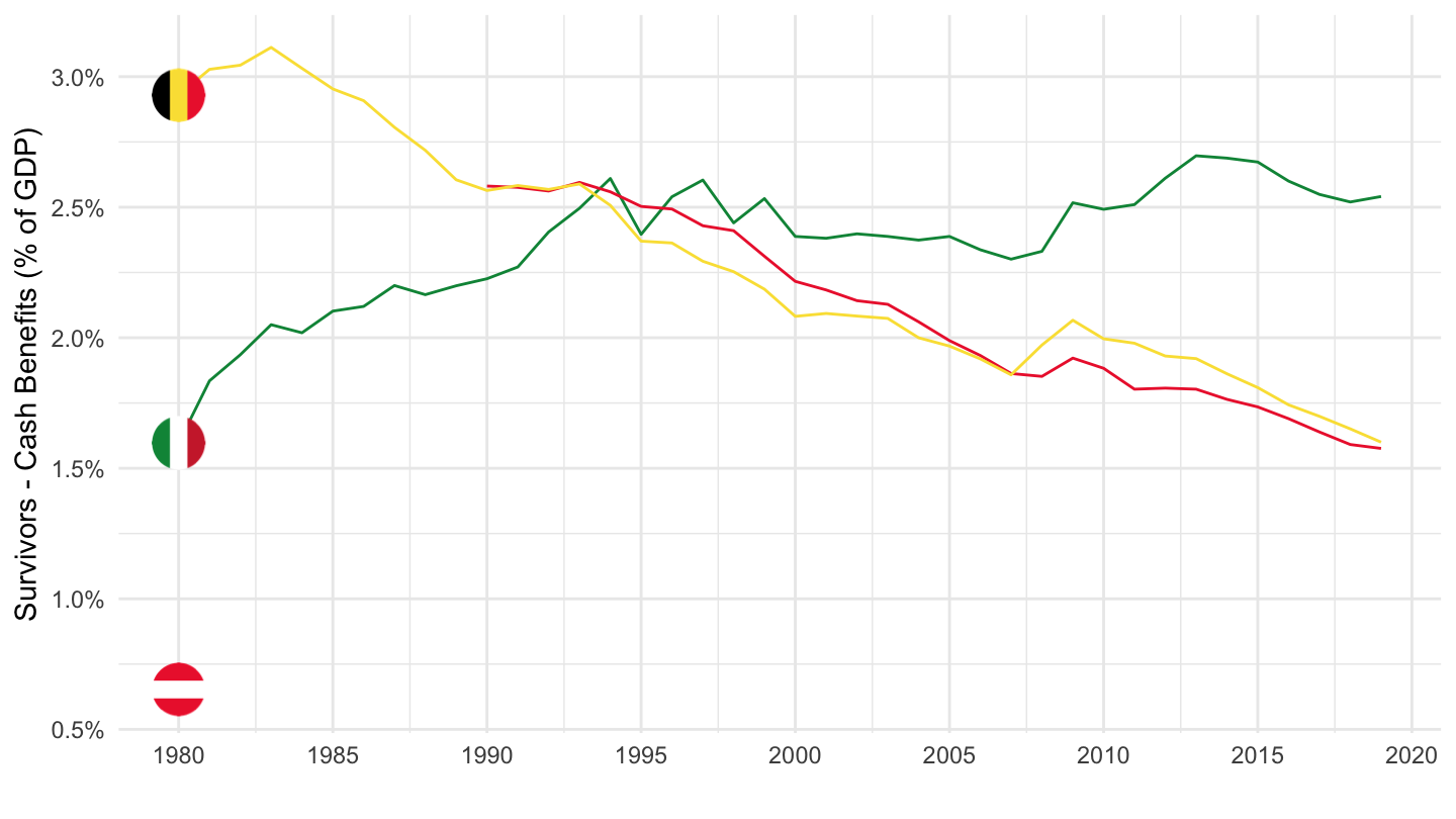
Health - Total (Branch 7)
World
Code
SOCX_AGG %>%
  filter(SOURCE == 10,
         TYPROG == 0,
         TYPEXP == 0,
         BRANCH == 4,
         UNIT == "PCT_GDP") %>%
  left_join(SOCX_AGG_var$COUNTRY, by = "COUNTRY") %>%
  year_to_enddate %>%
  mutate(year = year(date)) %>%
  filter(year %in% c(1990, 2000, 2015)) %>%
  arrange(Country, year) %>%
  group_by(Country, COUNTRY) %>%
  summarise(`1990 (% GDP)` = obsValue[1],
            `2000 (% GDP)` = obsValue[2],
            `2015 (% GDP)` = obsValue[3],
            `Delta 2000-15` = obsValue[3] - obsValue[2]) %>%
  arrange(-`2015 (% GDP)`) %>%
  mutate_at(vars(-Country, -COUNTRY), funs(round(., digits = 1))) %>%
  rename(`Country Name` = Country,
         `Country Code` = COUNTRY) -> SOC_AGG_BRANCH_4

# do.call(save, list("SOC_AGG_BRANCH_4", file = "SOC_AGG_BRANCH_4.RData"))

SOC_AGG_BRANCH_4 %>%
  {if (is_html_output()) datatable(., filter = 'top', rownames = F) else .}
United States, United Kingdom, Australia
Code
SOCX_AGG %>%
  filter(SOURCE == 10,
         TYPROG == 0,
         TYPEXP == 0,
         BRANCH == 4,
         UNIT == "PCT_GDP",
         COUNTRY %in% c("USA", "GBR", "AUS")) %>%
  left_join(SOCX_AGG_var$COUNTRY, by = "COUNTRY") %>%
  year_to_date %>%
  rename(Location = Country) %>%
  left_join(colors, by = c("Location" = "country")) %>%
  mutate(obsValue = obsValue / 100) %>%
  ggplot() + theme_minimal() + ylab("Health (% of GDP)") + xlab("") +
  geom_line(aes(x = date, y = obsValue, color = color)) +
  scale_color_identity() + add_3flags +
  scale_x_date(breaks = seq(1920, 2100, 5) %>% paste0("-01-01") %>% as.Date,
               labels = date_format("%Y")) +
  theme(legend.position = c(0.15, 0.9),
        legend.title = element_blank()) +
  scale_y_continuous(breaks = 0.01*seq(-7, 16, 0.5),
                     labels = scales::percent_format(accuracy = 0.1))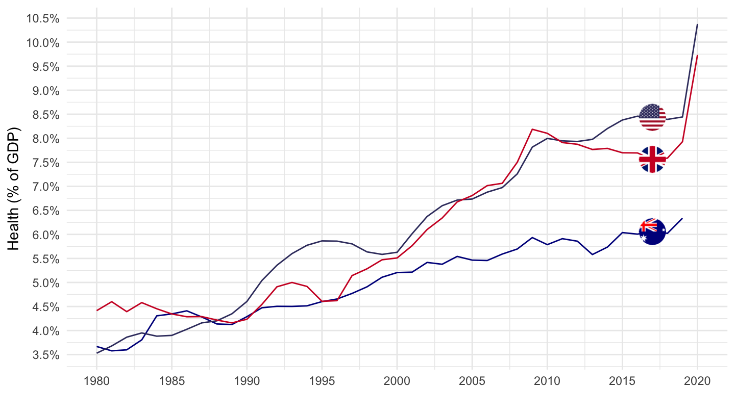
France, Germany, Netherlands
Code
SOCX_AGG %>%
  filter(SOURCE == 10,
         TYPROG == 0,
         TYPEXP == 0,
         BRANCH == 4,
         UNIT == "PCT_GDP",
         COUNTRY %in% c("FRA", "DEU", "NLD")) %>%
  left_join(SOCX_AGG_var$COUNTRY, by = "COUNTRY") %>%
  year_to_date %>%
  rename(Location = Country) %>%
  left_join(colors, by = c("Location" = "country")) %>%
  mutate(obsValue = obsValue / 100) %>%
  ggplot() + theme_minimal() + ylab("Health (% of GDP)") + xlab("") +
  geom_line(aes(x = date, y = obsValue, color = color)) +
  scale_color_identity() + add_3flags +
  scale_x_date(breaks = seq(1920, 2100, 5) %>% paste0("-01-01") %>% as.Date,
               labels = date_format("%Y")) +
  theme(legend.position = c(0.25, 0.9),
        legend.title = element_blank(),
        legend.direction = "horizontal") +
  scale_y_continuous(breaks = 0.01*seq(-7, 16, 0.5),
                     labels = scales::percent_format(accuracy = 0.1))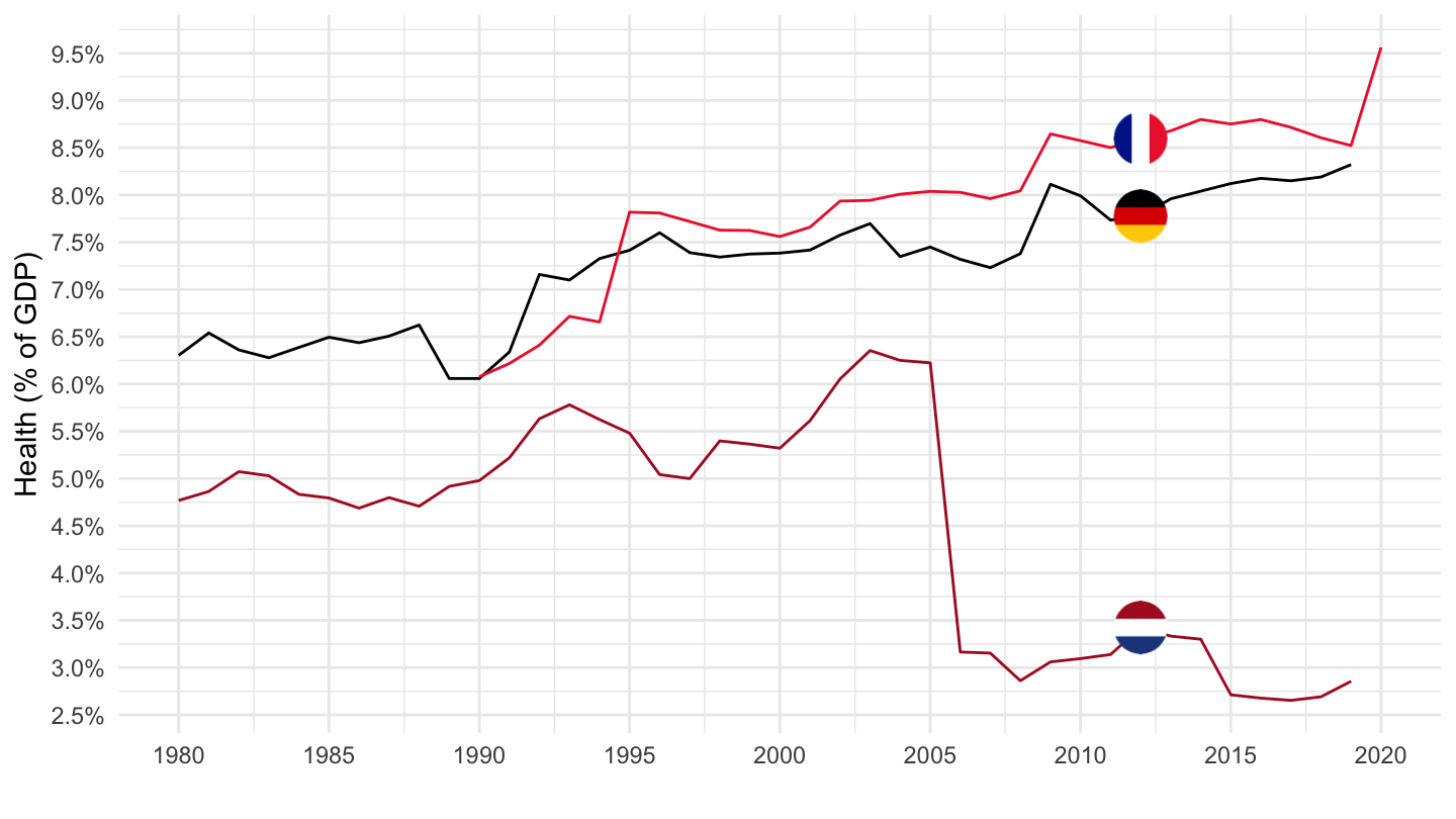
Chile, Denmark, Sweden
Code
SOCX_AGG %>%
  filter(SOURCE == 10,
         TYPROG == 0,
         TYPEXP == 0,
         BRANCH == 4,
         UNIT == "PCT_GDP",
         COUNTRY %in% c("DNK", "SWE", "CHL")) %>%
  left_join(SOCX_AGG_var$COUNTRY, by = "COUNTRY") %>%
  year_to_date %>%
  rename(Location = Country) %>%
  left_join(colors, by = c("Location" = "country")) %>%
  mutate(obsValue = obsValue / 100) %>%
  ggplot() + theme_minimal() + ylab("Health (% of GDP)") + xlab("") +
  geom_line(aes(x = date, y = obsValue, color = color)) +
  scale_color_identity() + add_3flags +
  scale_x_date(breaks = seq(1920, 2100, 5) %>% paste0("-01-01") %>% as.Date,
               labels = date_format("%Y")) +
  theme(legend.position = c(0.25, 0.2),
        legend.title = element_blank()) +
  scale_y_continuous(breaks = 0.01*seq(-7, 16, 0.5),
                     labels = scales::percent_format(accuracy = 0.1))
Switzerland, Canada, Slovenia
Code
SOCX_AGG %>%
  filter(SOURCE == 10,
         TYPROG == 0,
         TYPEXP == 0,
         BRANCH == 4,
         UNIT == "PCT_GDP",
         COUNTRY %in% c("CHE", "CAN", "SVN")) %>%
  left_join(SOCX_AGG_var$COUNTRY, by = "COUNTRY") %>%
  year_to_date %>%
  rename(Location = Country) %>%
  left_join(colors, by = c("Location" = "country")) %>%
  mutate(obsValue = obsValue / 100) %>%
  ggplot() + theme_minimal() + ylab("Health (% of GDP)") + xlab("") +
  geom_line(aes(x = date, y = obsValue, color = color)) +
  scale_color_identity() + add_3flags +
  scale_x_date(breaks = seq(1920, 2100, 5) %>% paste0("-01-01") %>% as.Date,
               labels = date_format("%Y")) +
  theme(legend.position = c(0.1, 0.85),
        legend.title = element_blank()) +
  scale_y_continuous(breaks = 0.01*seq(-7, 16, 0.5),
                     labels = scales::percent_format(accuracy = 0.1))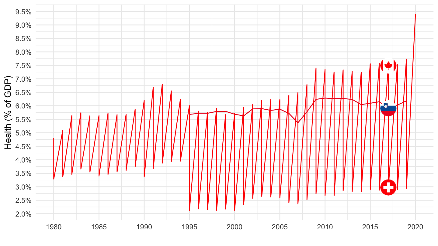
Austria, Belgium, Italy
Code
SOCX_AGG %>%
  filter(SOURCE == 10,
         TYPROG == 0,
         TYPEXP == 0,
         BRANCH == 4,
         UNIT == "PCT_GDP",
         COUNTRY %in% c("BEL", "AUT", "ITA")) %>%
  left_join(SOCX_AGG_var$COUNTRY, by = "COUNTRY") %>%
  year_to_date %>%
  rename(Location = Country) %>%
  left_join(colors, by = c("Location" = "country")) %>%
  mutate(obsValue = obsValue / 100) %>%
  ggplot() + theme_minimal() + ylab("Health (% of GDP)") + xlab("") +
  geom_line(aes(x = date, y = obsValue, color = color)) +
  scale_color_identity() + add_3flags +
  scale_x_date(breaks = seq(1920, 2100, 5) %>% paste0("-01-01") %>% as.Date,
               labels = date_format("%Y")) +
  theme(legend.position = c(0.15, 0.85),
        legend.title = element_blank()) +
  scale_y_continuous(breaks = 0.01*seq(-7, 16, 0.5),
                     labels = scales::percent_format(accuracy = 0.1))
Unemployment - Cash Benefits (Branch 7)
World
Code
SOCX_AGG %>%
  filter(SOURCE == 10,
         TYPROG == 0,
         TYPEXP == 1,
         BRANCH == 7,
         UNIT == "PCT_GDP") %>%
  left_join(SOCX_AGG_var$COUNTRY, by = "COUNTRY") %>%
  year_to_enddate %>%
  mutate(year = year(date)) %>%
  filter(year %in% c(1990, 2000, 2015)) %>%
  arrange(Country, year) %>%
  group_by(Country, COUNTRY) %>%
  summarise(`1990 (% GDP)` = obsValue[1],
            `2000 (% GDP)` = obsValue[2],
            `2015 (% GDP)` = obsValue[3],
            `Delta 2000-15` = obsValue[3] - obsValue[2]) %>%
  arrange(-`2015 (% GDP)`) %>%
  mutate_at(vars(-Country, -COUNTRY), funs(round(., digits = 1))) %>%
  rename(`Country Name` = Country,
         `Country Code` = COUNTRY) -> SOC_AGG_BRANCH_7

do.call(save, list("SOC_AGG_BRANCH_7", file = "SOC_AGG_BRANCH_7.RData"))

SOC_AGG_BRANCH_7 %>%
  {if (is_html_output()) datatable(., filter = 'top', rownames = F) else .}
France, Germany, Netherlands
Code
SOCX_AGG %>%
  filter(SOURCE == 10,
         TYPROG == 0,
         TYPEXP == 1,
         BRANCH == 7,
         UNIT == "PCT_GDP",
         COUNTRY %in% c("FRA", "DEU", "NLD")) %>%
  left_join(SOCX_AGG_var$COUNTRY, by = "COUNTRY") %>%
  year_to_date %>%
  rename(Location = Country) %>%
  left_join(colors, by = c("Location" = "country")) %>%
  mutate(obsValue = obsValue / 100) %>%
  ggplot() + theme_minimal() + ylab("Unemployment - Cash Benefits (% of GDP)") + xlab("") +
  geom_line(aes(x = date, y = obsValue, color = color)) +
  scale_color_identity() + add_3flags +
  scale_x_date(breaks = seq(1920, 2100, 5) %>% paste0("-01-01") %>% as.Date,
               labels = date_format("%Y")) +
  theme(legend.position = c(0.25, 0.9),
        legend.title = element_blank(),
        legend.direction = "horizontal") +
  scale_y_continuous(breaks = 0.01*seq(-7, 16, 0.5),
                     labels = scales::percent_format(accuracy = 0.1))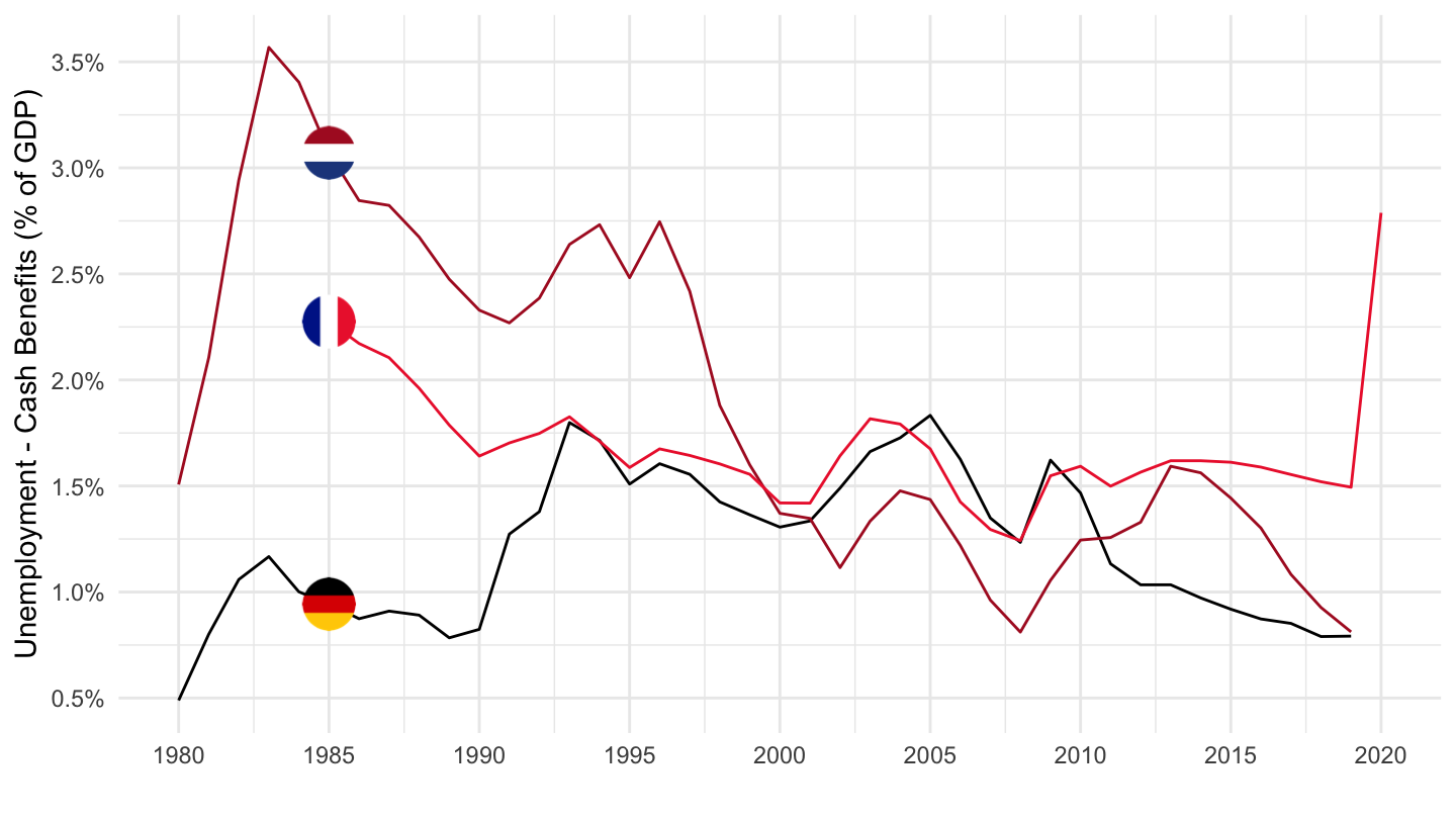
Chile, Denmark, Sweden
Code
SOCX_AGG %>%
  filter(SOURCE == 10,
         TYPROG == 0,
         TYPEXP == 1,
         BRANCH == 7,
         UNIT == "PCT_GDP",
         COUNTRY %in% c("DNK", "SWE", "CHL")) %>%
  left_join(SOCX_AGG_var$COUNTRY, by = "COUNTRY") %>%
  year_to_date %>%
  rename(Location = Country) %>%
  left_join(colors, by = c("Location" = "country")) %>%
  mutate(obsValue = obsValue / 100) %>%
  ggplot() + theme_minimal() + ylab("Unemployment - Cash Benefits (% of GDP)") + xlab("") +
  geom_line(aes(x = date, y = obsValue, color = color)) +
  scale_color_identity() + add_3flags +
  scale_x_date(breaks = seq(1920, 2100, 5) %>% paste0("-01-01") %>% as.Date,
               labels = date_format("%Y")) +
  theme(legend.position = c(0.25, 0.2),
        legend.title = element_blank()) +
  scale_y_continuous(breaks = 0.01*seq(-7, 16, 0.5),
                     labels = scales::percent_format(accuracy = 0.1))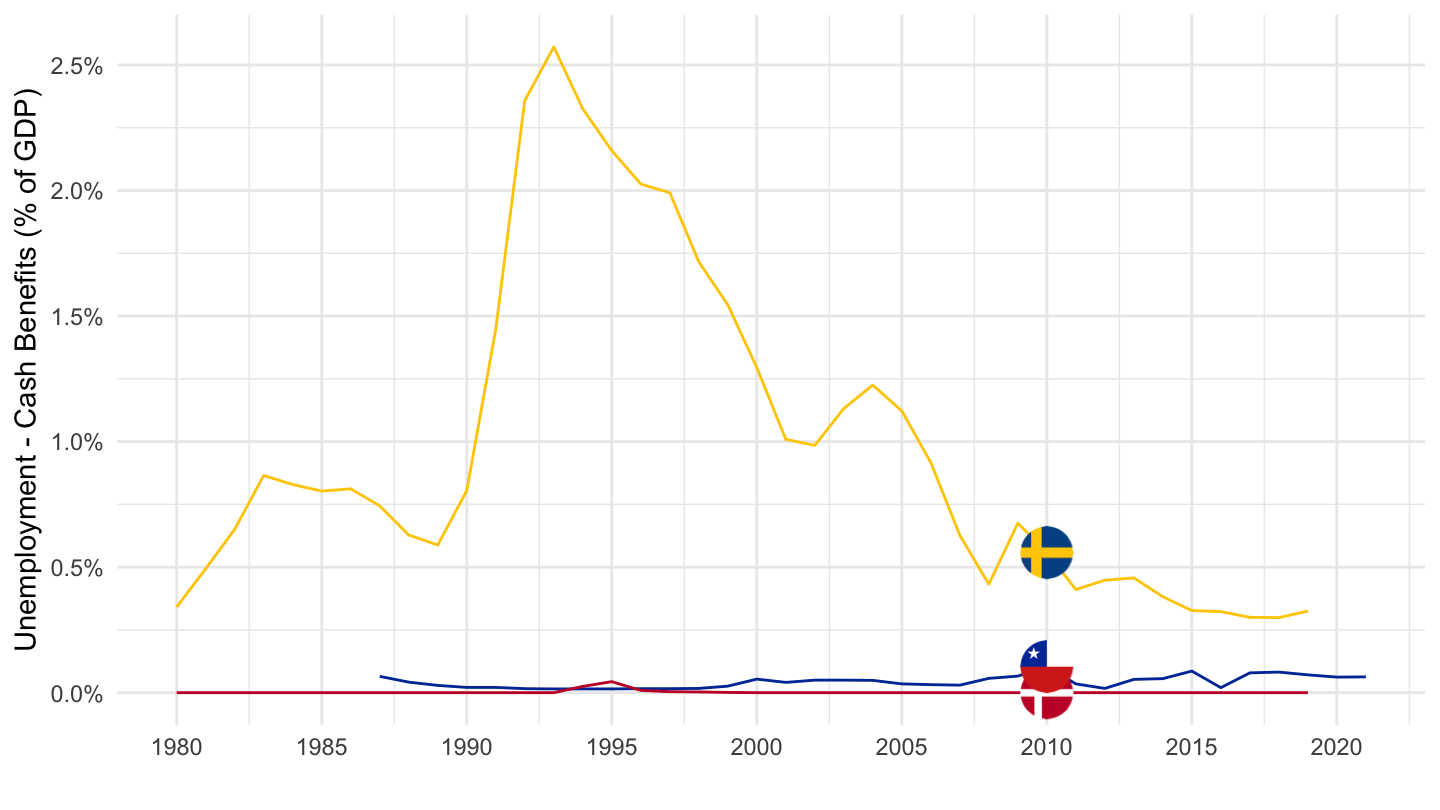
Switzerland, Canada, Sloveinia
Code
SOCX_AGG %>%
  filter(SOURCE == 10,
         TYPROG == 0,
         TYPEXP == 1,
         BRANCH == 7,
         UNIT == "PCT_GDP",
         COUNTRY %in% c("CHE", "CAN", "SVN")) %>%
  left_join(SOCX_AGG_var$COUNTRY, by = "COUNTRY") %>%
  year_to_date %>%
  rename(Location = Country) %>%
  left_join(colors, by = c("Location" = "country")) %>%
  mutate(obsValue = obsValue / 100) %>%
  ggplot() + theme_minimal() + ylab("Unemployment - Cash Benefits (% of GDP)") + xlab("") +
  geom_line(aes(x = date, y = obsValue, color = color)) +
  scale_color_identity() + add_3flags +
  scale_x_date(breaks = seq(1920, 2100, 5) %>% paste0("-01-01") %>% as.Date,
               labels = date_format("%Y")) +
  theme(legend.position = c(0.75, 0.85),
        legend.title = element_blank()) +
  scale_y_continuous(breaks = 0.01*seq(-7, 16, 0.5),
                     labels = scales::percent_format(accuracy = 0.1))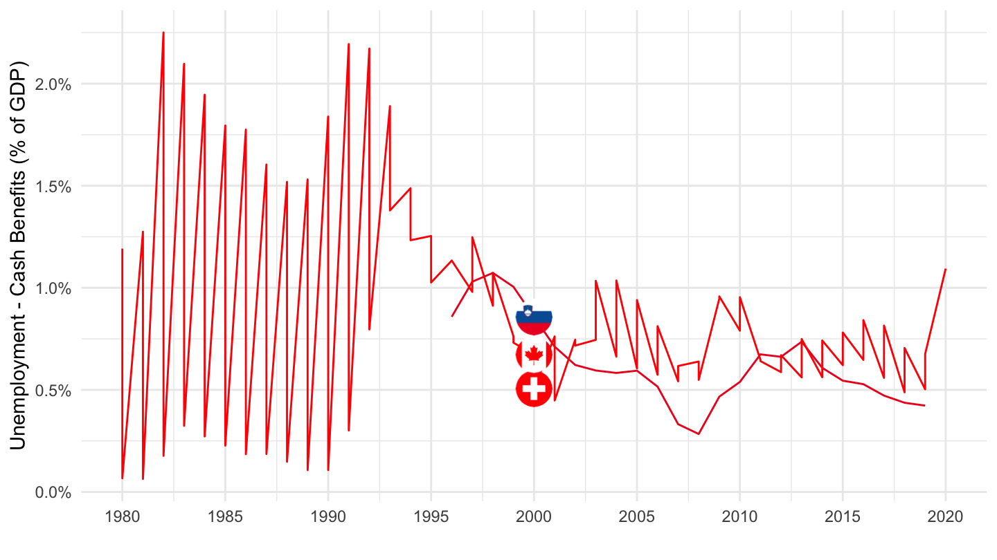
Austria, Belgium, Italy
Code
SOCX_AGG %>%
  filter(SOURCE == 10,
         TYPROG == 0,
         TYPEXP == 1,
         BRANCH == 7,
         UNIT == "PCT_GDP",
         COUNTRY %in% c("BEL", "AUT", "ITA")) %>%
  left_join(SOCX_AGG_var$COUNTRY, by = "COUNTRY") %>%
  year_to_date %>%
  rename(Location = Country) %>%
  left_join(colors, by = c("Location" = "country")) %>%
  mutate(obsValue = obsValue / 100) %>%
  ggplot() + theme_minimal() + ylab("Unemployment - Cash Benefits (% of GDP)") + xlab("") +
  geom_line(aes(x = date, y = obsValue, color = color)) +
  scale_color_identity() + add_3flags +
  scale_x_date(breaks = seq(1920, 2100, 5) %>% paste0("-01-01") %>% as.Date,
               labels = date_format("%Y")) +
  theme(legend.position = c(0.15, 0.85),
        legend.title = element_blank()) +
  scale_y_continuous(breaks = 0.01*seq(-7, 16, 1),
                     labels = scales::percent_format(accuracy = 0.1))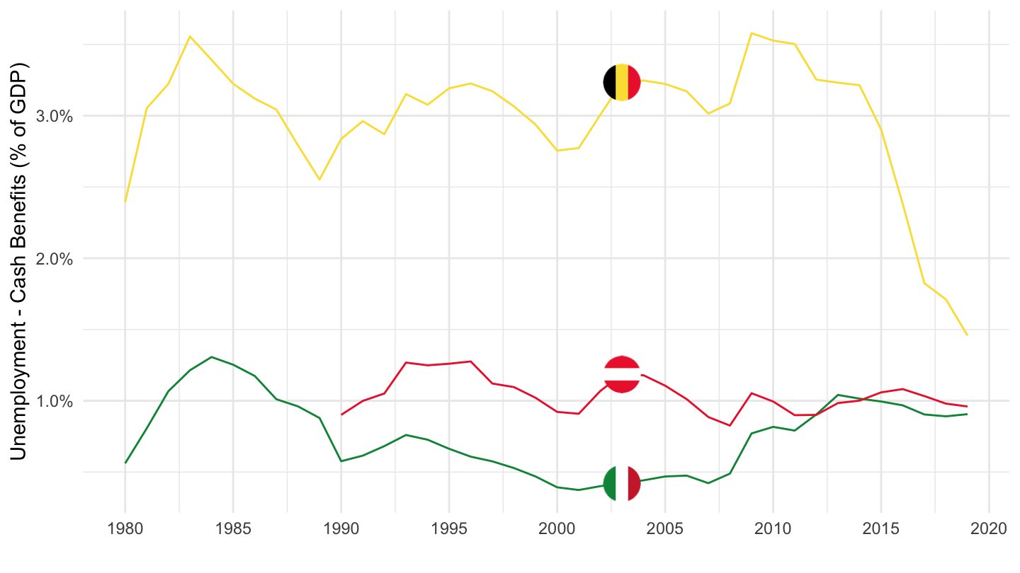
France and Germany
Total - Old Age
Code
SOCX_AGG %>%
  filter(SOURCE == 10,
         TYPROG == 0,
         TYPEXP == 1,
         BRANCH == 1,
         UNIT == "PCT_GDP",
         COUNTRY %in% c("FRA", "DEU")) %>%
  left_join(SOCX_AGG_var$COUNTRY, by = "COUNTRY") %>%
  left_join(SOCX_AGG_var$BRANCH, by = "BRANCH") %>%
  left_join(SOCX_AGG_var$TYPEXP, by = "TYPEXP") %>%
  mutate(date = paste0(obsTime, "-01-01") %>% as.Date,
         value = obsValue / 100) %>%
  filter(year(date) >= 1990) %>%
  arrange(Country) %>%
  select(Branch, Country, Typexp, date, value) %>%
  mutate(Variable = paste0(Branch, " - ", Typexp, " (", Country, ")")) %>%
  ggplot() + geom_line(aes(x = date, y = value, color = Variable)) +
  scale_color_manual(values = viridis(3)[1:2]) +
  theme_minimal() +
  scale_x_date(breaks = seq(1920, 2100, 2) %>% paste0("-01-01") %>% as.Date,
               labels = date_format("%Y")) +
  theme(legend.position = c(0.25, 0.9),
        legend.title = element_blank()) +
  scale_y_continuous(breaks = 0.01*seq(-7, 16, 0.5),
                     labels = scales::percent_format(accuracy = 0.1)) +
  ylab("% of GDP") + xlab("")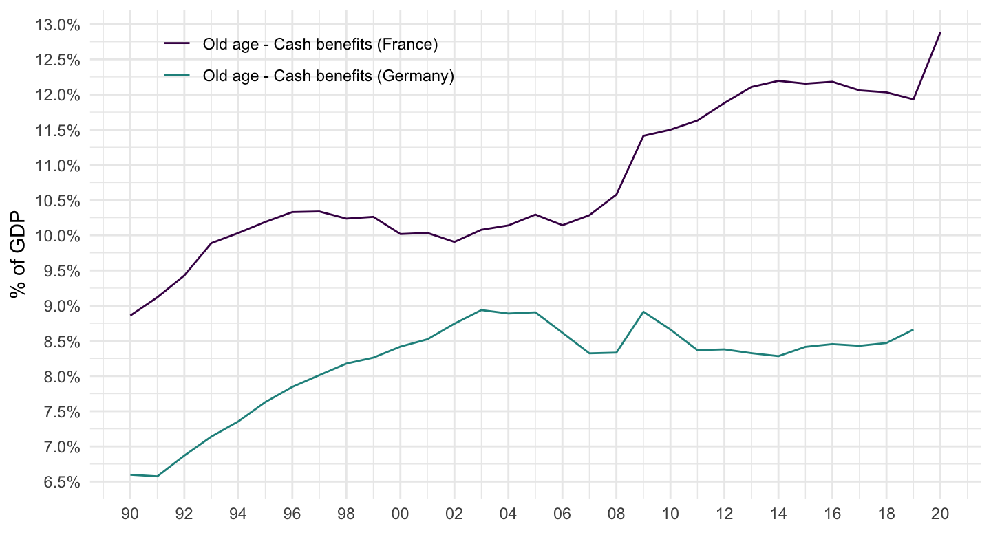
Old age - Cash benefits
Code
SOCX_AGG %>%
  filter(SOURCE == 10,
         TYPROG == 0,
         TYPEXP == 1,
         BRANCH == 1,
         UNIT == "PCT_GDP",
         COUNTRY %in% c("FRA", "DEU")) %>%
  left_join(SOCX_AGG_var$COUNTRY, by = "COUNTRY") %>%
  left_join(SOCX_AGG_var$BRANCH, by = "BRANCH") %>%
  left_join(SOCX_AGG_var$TYPEXP, by = "TYPEXP") %>%
  mutate(date = paste0(obsTime, "-01-01") %>% as.Date,
         value = obsValue / 100) %>%
  filter(year(date) >= 1990) %>%
  arrange(Country) %>%
  select(Branch, Country, Typexp, date, value) %>%
  mutate(Variable = paste0(Branch, " - ", Typexp, " (", Country, ")")) %>%
  ggplot() + geom_line(aes(x = date, y = value, color = Variable)) +
  scale_color_manual(values = viridis(3)[1:2]) +
  theme_minimal() +
  scale_x_date(breaks = seq(1920, 2100, 2) %>% paste0("-01-01") %>% as.Date,
               labels = date_format("%Y")) +
  theme(legend.position = c(0.25, 0.8),
        legend.title = element_blank()) +
  scale_y_continuous(breaks = 0.01*seq(-7, 16, 0.5),
                     labels = scales::percent_format(accuracy = 0.1)) +
  ylab("% of GDP") + xlab("")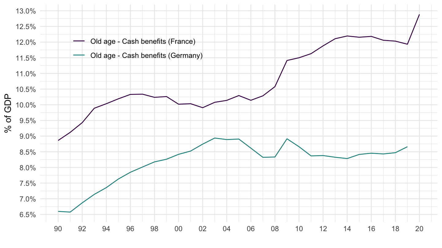
Total - Cash Benefits
Code
SOCX_AGG %>%
  filter(SOURCE == 10,
         TYPROG == 0,
         TYPEXP == 1,
         BRANCH == 90,
         UNIT == "PCT_GDP",
         COUNTRY %in% c("FRA", "DEU")) %>%
  left_join(SOCX_AGG_var$COUNTRY, by = "COUNTRY") %>%
  left_join(SOCX_AGG_var$BRANCH, by = "BRANCH") %>%
  left_join(SOCX_AGG_var$TYPEXP, by = "TYPEXP") %>%
  mutate(date = paste0(obsTime, "-01-01") %>% as.Date,
         value = obsValue / 100) %>%
  filter(year(date) >= 1990) %>%
  arrange(Country) %>%
  select(Branch, Country, Typexp, date, value) %>%
  mutate(Variable = paste0(Branch, " - ", Typexp, " (", Country, ")")) %>%
  ggplot() + geom_line(aes(x = date, y = value, color = Variable)) +
  scale_color_manual(values = viridis(3)[1:2]) +
  theme_minimal() +
  scale_x_date(breaks = seq(1920, 2100, 2) %>% paste0("-01-01") %>% as.Date,
               labels = date_format("%Y")) +
  theme(legend.position = c(0.25, 0.7),
        legend.title = element_blank()) +
  scale_y_continuous(breaks = 0.01*seq(-7, 26, 0.5),
                     labels = scales::percent_format(accuracy = 0.1)) +
  ylab("% of GDP") + xlab("")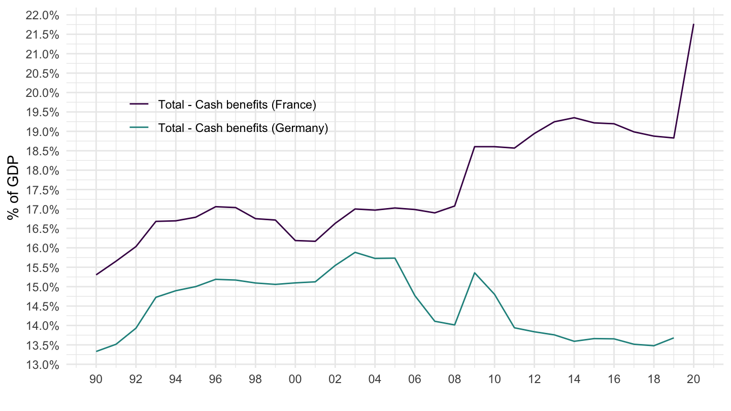
Health - Total
Code
SOCX_AGG %>%
  filter(SOURCE == 10,
         TYPROG == 0,
         TYPEXP == 0,
         BRANCH == 4,
         UNIT == "PCT_GDP",
         COUNTRY %in% c("FRA", "DEU")) %>%
  left_join(SOCX_AGG_var$COUNTRY, by = "COUNTRY") %>%
  left_join(SOCX_AGG_var$BRANCH, by = "BRANCH") %>%
  left_join(SOCX_AGG_var$TYPEXP, by = "TYPEXP") %>%
  mutate(date = paste0(obsTime, "-01-01") %>% as.Date,
         value = obsValue / 100) %>%
  filter(year(date) >= 1990) %>%
  arrange(Country) %>%
  select(Branch, Country, Typexp, date, value) %>%
  mutate(Variable = paste0(Branch, " - ", Typexp, " (", Country, ")")) %>%
  ggplot() + geom_line(aes(x = date, y = value, color = Variable)) +
  scale_color_manual(values = viridis(3)[1:2]) +
  theme_minimal() +
  scale_x_date(breaks = seq(1920, 2100, 2) %>% paste0("-01-01") %>% as.Date,
               labels = date_format("%Y")) +
  theme(legend.position = c(0.15, 0.9),
        legend.title = element_blank()) +
  scale_y_continuous(breaks = 0.01*seq(-7, 26, 0.5),
                     labels = scales::percent_format(accuracy = 0.1)) +
  ylab("% of GDP") + xlab("")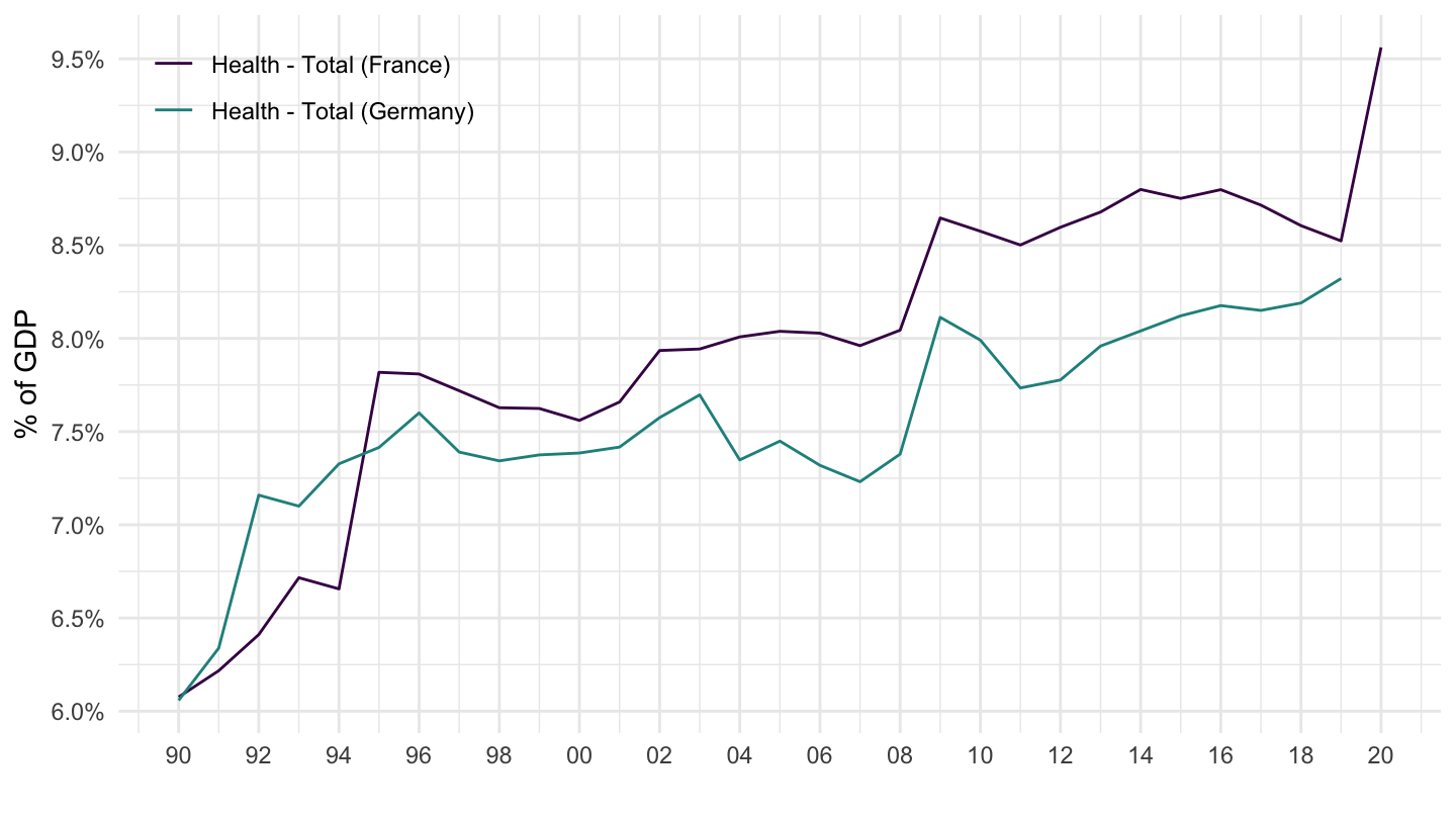
Family - Total
Code
SOCX_AGG %>%
  filter(SOURCE == 10,
         TYPROG == 0,
         TYPEXP == 0,
         BRANCH == 5,
         UNIT == "PCT_GDP",
         COUNTRY %in% c("FRA", "DEU")) %>%
  left_join(SOCX_AGG_var$COUNTRY, by = "COUNTRY") %>%
  left_join(SOCX_AGG_var$BRANCH, by = "BRANCH") %>%
  left_join(SOCX_AGG_var$TYPEXP, by = "TYPEXP") %>%
  mutate(date = paste0(obsTime, "-01-01") %>% as.Date,
         value = obsValue / 100) %>%
  filter(year(date) >= 1990) %>%
  arrange(Country) %>%
  select(Branch, Country, Typexp, date, value) %>%
  mutate(Variable = paste0(Branch, " - ", Typexp, " (", Country, ")")) %>%
  ggplot() + geom_line(aes(x = date, y = value, color = Variable)) +
  scale_color_manual(values = viridis(3)[1:2]) +
  theme_minimal() +
  scale_x_date(breaks = seq(1920, 2100, 2) %>% paste0("-01-01") %>% as.Date,
               labels = date_format("%Y")) +
  theme(legend.position = c(0.15, 0.9),
        legend.title = element_blank()) +
  scale_y_continuous(breaks = 0.01*seq(-7, 26, 0.2),
                     labels = scales::percent_format(accuracy = 0.1)) +
  ylab("% of GDP") + xlab("")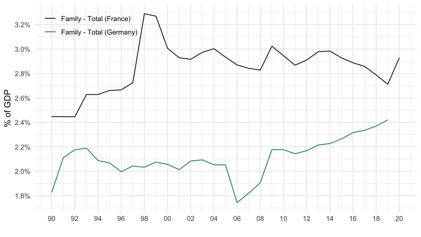
Housing - Total
Code
SOCX_AGG %>%
  filter(SOURCE == 10,
         TYPROG == 0,
         TYPEXP == 0,
         BRANCH == 8,
         UNIT == "PCT_GDP",
         COUNTRY %in% c("FRA", "DEU")) %>%
  left_join(SOCX_AGG_var$COUNTRY, by = "COUNTRY") %>%
  left_join(SOCX_AGG_var$BRANCH, by = "BRANCH") %>%
  left_join(SOCX_AGG_var$TYPEXP, by = "TYPEXP") %>%
  mutate(date = paste0(obsTime, "-01-01") %>% as.Date,
         value = obsValue / 100) %>%
  filter(year(date) >= 1990) %>%
  arrange(Country) %>%
  select(Branch, Country, Typexp, date, value) %>%
  mutate(Variable = paste0(Branch, " - ", Typexp, " (", Country, ")")) %>%
  ggplot() + geom_line(aes(x = date, y = value, color = Variable)) +
  scale_color_manual(values = viridis(3)[1:2]) +
  theme_minimal() +
  scale_x_date(breaks = seq(1920, 2100, 2) %>% paste0("-01-01") %>% as.Date,
               labels = date_format("%Y")) +
  theme(legend.position = c(0.2, 0.5),
        legend.title = element_blank()) +
  scale_y_continuous(breaks = 0.01*seq(-7, 26, 0.1),
                     labels = scales::percent_format(accuracy = 0.1)) +
  ylab("% of GDP") + xlab("")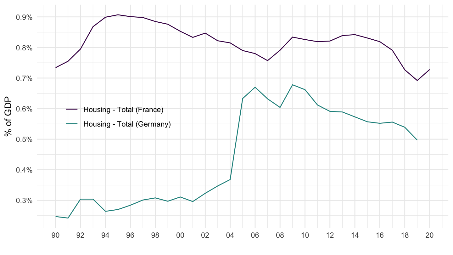
10-112
Code
SOCX_AGG %>%
  filter(SOURCE == 10,
         TYPROG == 112,
         TYPEXP == 1,
         BRANCH == 1,
         UNIT == "PCT_GDP",
         COUNTRY %in% c("FRA", "DEU")) %>%
  left_join(SOCX_AGG_var$COUNTRY, by = "COUNTRY") %>%
  mutate(date = paste0(obsTime, "-01-01") %>% as.Date,
         value = obsValue / 100) %>%
  arrange(Country) %>%
  select(Country, date, value) %>%
  ggplot() + geom_line(aes(x = date, y = value, color = Country)) +
  scale_color_manual(values = viridis(3)[1:2]) +
  theme_minimal() +
  scale_x_date(breaks = seq(1920, 2100, 2) %>% paste0("-01-01") %>% as.Date,
               labels = date_format("%Y")) +
  theme(legend.position = c(0.25, 0.4),
        legend.title = element_blank()) +
  scale_y_continuous(breaks = 0.01*seq(-7, 2, 0.1),
                     labels = scales::percent_format(accuracy = 0.1)) +
  ylab("% of GDP") + xlab("")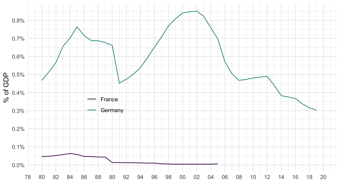
Old age - Cash benefits
France, Germany, Netherlands
Code
SOCX_AGG %>%
  filter(SOURCE == 10,
         TYPROG == 0,
         TYPEXP == 1,
         BRANCH == 1,
         UNIT == "PCT_GDP",
         COUNTRY %in% c("FRA", "DEU", "NLD")) %>%
  left_join(SOCX_AGG_var$COUNTRY, by = "COUNTRY") %>%
  left_join(SOCX_AGG_var$BRANCH, by = "BRANCH") %>%
  left_join(SOCX_AGG_var$TYPEXP, by = "TYPEXP") %>%
  mutate(date = paste0(obsTime, "-01-01") %>% as.Date,
         value = obsValue / 100) %>%
  filter(year(date) >= 1990) %>%
  arrange(Country) %>%
  select(Branch, Country, Typexp, date, value) %>%
  mutate(Variable = paste0(Branch, " - ", Typexp, " (", Country, ")")) %>%
  ggplot() + geom_line(aes(x = date, y = value, color = Variable)) +
  scale_color_manual(values = viridis(4)[1:3]) +
  theme_minimal() +
  scale_x_date(breaks = seq(1920, 2100, 2) %>% paste0("-01-01") %>% as.Date,
               labels = date_format("%Y")) +
  theme(legend.position = c(0.25, 0.9),
        legend.title = element_blank()) +
  scale_y_continuous(breaks = 0.01*seq(-7, 16, 0.5),
                     labels = scales::percent_format(accuracy = 0.1)) +
  ylab("% of GDP") + xlab("")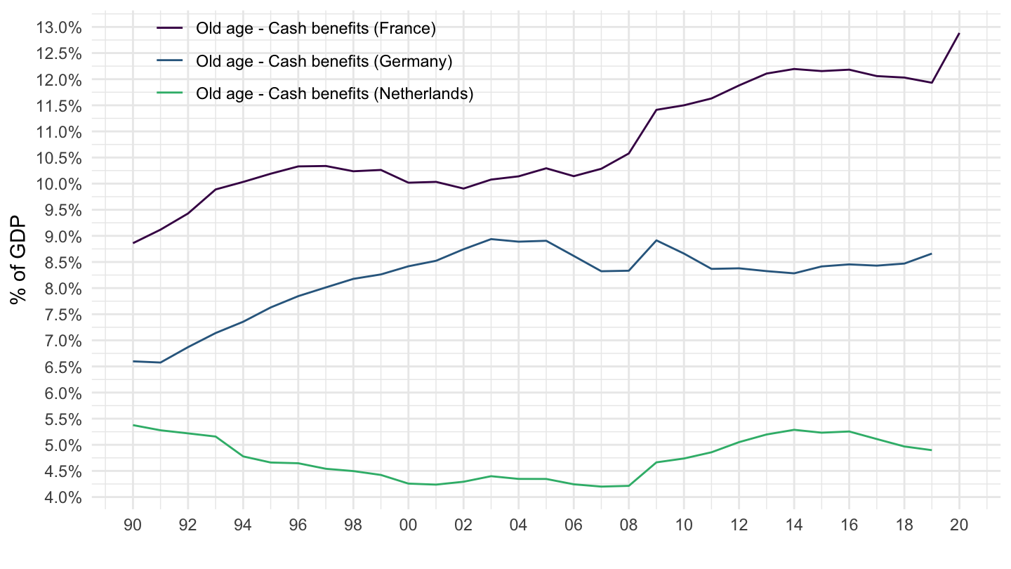
Belgium, Austria, Italy
Code
SOCX_AGG %>%
  filter(SOURCE == 10,
         TYPROG == 0,
         TYPEXP == 1,
         BRANCH == 1,
         UNIT == "PCT_GDP",
         COUNTRY %in% c("BEL", "AUT", "ITA")) %>%
  left_join(SOCX_AGG_var$COUNTRY, by = "COUNTRY") %>%
  left_join(SOCX_AGG_var$BRANCH, by = "BRANCH") %>%
  left_join(SOCX_AGG_var$TYPEXP, by = "TYPEXP") %>%
  mutate(date = paste0(obsTime, "-01-01") %>% as.Date,
         value = obsValue / 100) %>%
  filter(year(date) >= 1980) %>%
  arrange(Country) %>%
  select(Branch, Country, Typexp, date, value) %>%
  mutate(Variable = paste0(Branch, " - ", Typexp, " (", Country, ")")) %>%
  ggplot() + geom_line(aes(x = date, y = value, color = Variable)) +
  scale_color_manual(values = viridis(4)[1:3]) +
  theme_minimal() +
  scale_x_date(breaks = seq(1920, 2100, 2) %>% paste0("-01-01") %>% as.Date,
               labels = date_format("%Y")) +
  theme(legend.position = c(0.25, 0.9),
        legend.title = element_blank()) +
  scale_y_continuous(breaks = 0.01*seq(-7, 16, 0.5),
                     labels = scales::percent_format(accuracy = 0.1)) +
  ylab("% of GDP") + xlab("")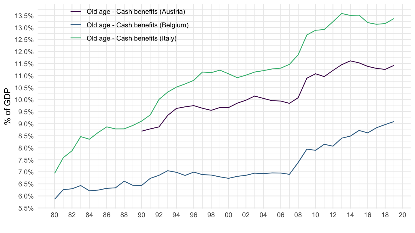
Social aggregate, Public
World
Code
World
Code
Code