The Phillips Curve Is Not What You Think
inflation
Phillips curve
[🌐 HTML Presentation] [🎞️ PDF Presentation] [📄 PDF Article]
The Covid-19 crisis has brought stimulus policy back to the centre of macroeconomic debate. In the United States, a number of economists have warned that the Biden administration’s $1.9 trillion fiscal package risks driving unemployment below its sustainable level and triggering an inflationary spiral - what is commonly termed an “overheating” effect. In Europe, the prevailing concern runs in the opposite direction: that current stimulus measures are inadequate to prevent unemployment from remaining durably elevated, thereby exposing the economy to deflationary pressures. Despite their divergent conclusions, both positions rest on a shared analytical premise - the existence of a Phillips curve, understood as an inverse relationship between the unemployment rate and the rate of inflation. This cornerstone of macroeconomic theory has, however, been subject to sustained empirical scrutiny. Economic history furnishes numerous episodes in which the expected unemployment–inflation trade-off proves difficult to identify, casting doubt on the robustness of the relationship. Does this imply that the Phillips curve should be relegated to the growing list of economic regularities that have ceased to hold? In its conventional formulation, the answer may well be yes. However, a reformulation grounded in empirical observation suggests a more productive alternative: what underlies the Phillips curve is, in fact, a negative relationship between unemployment and real exchange rate appreciation - a variable that coincides with inflation under fixed exchange rate regimes, thereby generating the observed correlation (Geerolf 2018). This reinterpretation carries significant implications for economic policy. First, it reframes the relevant trade-off as one between external competitiveness and unemployment, rather than between inflation and unemployment per se. Second, it undermines the use of the inflation rate as a reliable guide for macroeconomic stabilisation: inflation is not a sufficient indicator of excess demand, nor is its absence evidence that demand is adequate. Third, and perhaps most consequentially, it calls into question the notion of a natural rate of unemployment below which inflationary pressures would inevitably materialise, as was widely assumed since the 1970s and 1980s. Taken together, these considerations suggest that current anxieties surrounding the inflationary risks of fiscal stimulus deserve to be treated with considerable caution.
The Phillips Curve: An Empirically Contested Pillar of Macroeconomics
In the late 1950s, the economist A.W. Phillips identified a downward-sloping relationship between the unemployment rate and the growth of nominal wages in Great Britain between 1861 and 1913 (Phillips 1958). A straightforward explanation was soon proposed: when unemployment is low, firms face recruitment difficulties, leading them to offer higher nominal wages; conversely, in periods of elevated unemployment, bargaining power shifts away from workers, resulting in wage moderation. On the further assumption of a direct link between nominal wage growth and inflation, this implies a negative relationship between unemployment and the price level more broadly.1
The Phillips curve rapidly became a cornerstone of macroeconomic theory. As early as 1960, Paul Samuelson and Robert Solow, having identified an analogous relationship in the United States, amplified Phillips’s contribution by placing the curve at the heart of the “neoclassical synthesis” - the theoretical bridge between Keynesian and neoclassical economics. Within this framework, the economy is conceived as Keynesian in the short run and neoclassical in the long run. The Phillips curve gives concrete form to the trade-off between unemployment and inflation, and to the short-run policy dilemma facing governments: any feasible combination of unemployment and inflation rates is constrained by the observation that lower unemployment comes at the cost of higher inflation.
Despite repeated empirical challenges, the Phillips curve has demonstrated remarkable theoretical resilience, with each critique giving rise to a reformulation that preserves its core logic.2 The most influential such reformulation was advanced by Edmund Phelps and Milton Friedman in the late 1960s. In their account, the underlying relationship - known as the expectations-augmented Phillips curve - links changes in the rate of inflation to the gap between actual unemployment and the so-called natural rate: the unemployment rate consistent with stable inflation, or Non-Accelerating Inflation Rate of Unemployment (NAIRU). This respecification proved considerably less hospitable to Keynesian policy prescriptions, since any demand-side stimulus aimed at pushing unemployment below its natural level would, on this view, produce ever-accelerating inflation3. Moreover, empirical estimates of the NAIRU have typically been high: the 2000 report Full Employment by the French Council of Economic Analysis, for instance, placed it at between 8% and 10% in France (Pisani-Ferry et al. 2000). From a policy standpoint, the augmented Phillips curve provided, from the 1990s onwards, the analytical foundation both for inflation-targeting monetary frameworks and for structural labour market reforms oriented towards greater flexibility - widely regarded as the principal lever for reducing the natural rate of unemployment.
The expectations-augmented curve nevertheless proved empirically disappointing from the 1980s onwards. Confronted with its numerous shortcomings - particularly its failure to account for the persistence of unemployment in Europe - Larry Summers posed the question directly in 1991: “Should Keynesian economics dispense with the Phillips curve?” (Summers 1991).
In the late 1990s, unemployment in the United States fell well below prevailing NAIRU estimates during the dot-com boom, yet generated no discernible inflationary pressure. During the 2000s, both the European Central Bank and the Federal Reserve tightened monetary policy on multiple occasions as unemployment appeared to approach its natural level, even in the absence of any visible inflationary tensions. The severity of the 2007–2009 crisis, and the sharp rise in unemployment it produced, did not give rise to the deflationary dynamics that standard models would have predicted. Nor did the fiscal expansion under the Trump administration (2017–2020) prove inflationary. If the Phillips curve - despite successive theoretical refinements - repeatedly vanishes from the empirical landscape, the question arises whether the underlying premise of a stable relationship between unemployment and prices ought to be abandoned altogether.
A Solid Pillar: The Exchange-Rate Phillips Curve
In its traditional formulations, it is difficult to sustain the claim that a stable relationship between unemployment and inflation exists. However, when unemployment is related not to inflation but to changes in the real exchange rate - that is, to relative inflation expressed in a common currency - a stable negative relationship between unemployment and real exchange rate appreciation does emerge (Geerolf 2018).
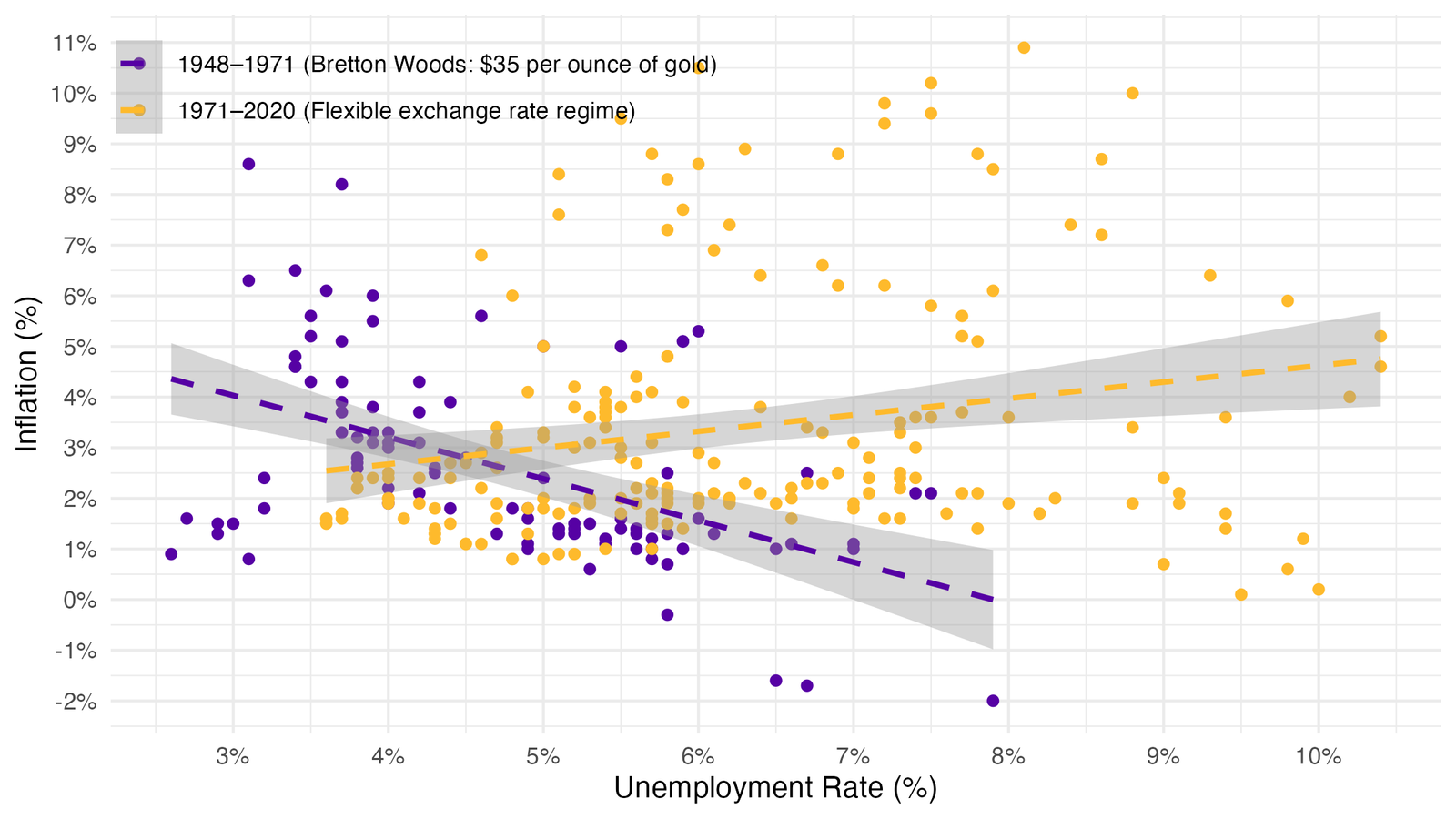
Under fixed exchange rate regimes, this reinterpretation does not contradict Phillips’s original findings, since inflation and real exchange rate appreciation coincide by definition in such regimes. This accounts for the existence of a Phillips curve in economies operating under fixed exchange rates, such as Great Britain between 1861 and 1913 (under the gold standard) or the United States, which occupied the centre of the Bretton Woods system until 1971 (Figure 1). By the same logic, Phillips curves are regularly identified at the sub-national level - across U.S. states, regions within a given country, member states of the euro area, or economies sharing a common currency.4
As Figure 2 based on Geerolf (2018) and Ilzetzki et al. (2019) illustrates more broadly, a clear negative relationship between unemployment and inflation is indeed observable among OECD countries operating under fixed exchange rate regimes over the period 1960–2016.
Under flexible exchange rate regimes, by contrast, the correlation between inflation and unemployment is positive, which invalidates the traditional Phillips curve. Recovering a negative relationship between unemployment and prices - irrespective of the exchange rate regime - requires moving away from overall inflation and focusing instead on relative inflation: that of non-tradable goods relative to tradable goods, that is, changes in the real exchange rate.
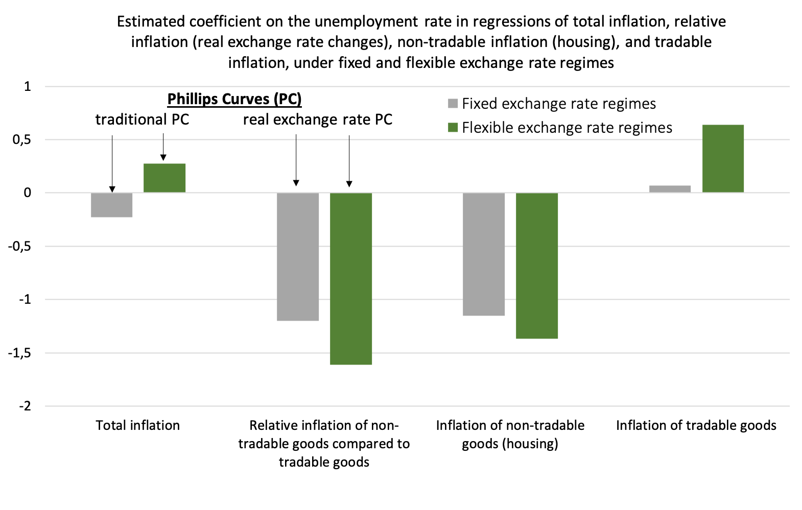
Decomposing the effect of the unemployment rate on inflation into its two components - non-tradable goods and tradable goods - helps account for this pattern.
Under both fixed and flexible exchange rate regimes, a demand-driven decline in unemployment generates upward pressure on demand for non-tradable goods, whose supply is relatively inelastic. Their prices consequently rise - a dynamic particularly pronounced in housing and rental markets. The relationship between unemployment and inflation in non-tradable goods is therefore negative under either regime.
For tradable goods, the relationship between unemployment and inflation depends on the prevailing exchange rate regime. Under fixed exchange rates, the relationship is negligible: since prices are determined on global markets and the exchange rate does not adjust, there is no systematic mechanism linking unemployment to tradable goods inflation. Under flexible exchange rates, however, the relationship is positive: a decline in unemployment tends to be accompanied by nominal exchange rate appreciation, which depresses the domestic-currency price of tradable goods. This appreciation reflects central bank intervention aimed at containing inflationary pressure: as falling unemployment drives up non-tradable goods prices, central banks respond by tightening monetary policy, which, under flexible exchange rates, induces currency appreciation. The relationship between unemployment and tradable goods inflation is therefore either negligible or positive.
Since the traditional Phillips curve relates unemployment to overall inflation - a weighted average of inflation in tradable and non-tradable goods - it is more likely to be observed under fixed exchange rates, where the relationship is negative for non-tradables and negligible for tradables. Under flexible exchange rates, if the positive effect of unemployment on tradable goods inflation - weighted by the tradable share of consumption - outweighs the negative effect on non-tradable goods inflation, the traditional Phillips curve is reversed.
The exchange-rate Phillips curve, by contrast, holds regardless of the exchange rate regime, as it relates unemployment to the relative inflation of non-tradable goods with respect to tradable goods - a relationship that is robustly negative across regimes.
The Exchange-Rate Phillips Curve Offers a Different View of Economic Policy
The exchange-rate Phillips curve carries significant implications for the conduct of economic policy. First, it establishes that the relevant trade-off is not between lower unemployment and lower inflation, but between lower unemployment and external competitiveness. This implies that the risks associated with demand stimulus are not inflationary in nature, but concern rather the erosion of export sector competitiveness - entailing a reallocation of production away from manufacturing and towards construction and non-tradable services, and thereby accelerating deindustrialisation.5 This tension between fiscal stimulus and competitive deterioration has confronted policymakers on numerous occasions. The decline in U.S. competitiveness following the Keynesian policies of the 1960s was among the considerations that led Richard Nixon to devalue the dollar in 1971.6 Analogous dynamics have been observed in emerging economies - Argentina between 1991 and 2000, and Southeast Asia during the 1990s - as well as in Southern Europe, where Greece, Spain, and Ireland experienced similar pressures in the early 2000s. This problem arises, however, only in the case of uncoordinated stimulus, and thus argues in favour of internationally coordinated fiscal expansion, of the kind implemented at the G20 summit in Washington in 2008. The tension between demand stimulus and external balance was already central to Keynes’s own thinking: he advocated the use of tariffs to mitigate these effects in the absence of coordinated action.7
The absence of a traditional Phillips curve further implies that the inflation rate is not a reliable guide for macroeconomic policy, and that stabilising inflation is neither necessary nor sufficient to stabilise economic activity. The stagflation of the 1970s, for instance, was interpreted at the time as a symptom of excess demand - since, under the traditional Phillips curve, deficient demand should have produced deflation - and this interpretation furnished the justification for the austerity policies that followed, notably the sharp tightening of U.S. monetary policy in the 1980s. The exchange-rate Phillips curve, however, offers an alternative reading: the coexistence of unemployment and inflation during that period is consistent with deficient demand once one recognises that it reflected the real depreciation of the dollar consequent on its nominal devaluation at the end of the Bretton Woods system.
By the same logic, the “missing deflation” of 2007–2009 does not imply that the financial crisis was accompanied by a positive supply shock - contrary to what a New Keynesian framework relying on the traditional Phillips curve would suggest.8 Similarly, the European Central Bank’s interest rate increases in 2011 were unnecessary: the observed rise in inflation was not a sign of overheating in an economy that was, in fact, undergoing substantial fiscal consolidation between 2010 and 2013, but rather the consequence of euro depreciation and the imported inflation it generated - precisely the mechanism described by the exchange-rate Phillips curve. The subsequent absence of deflation is not inconsistent with the fact that economic activity in Europe has remained persistently below potential, particularly in comparison with the United States.
Finally, the absence of a Phillips curve linking unemployment to inflation calls into question the standard objections to demand-support policies. The debates surrounding the limits of fiscal stimulus - which remain live in current discussions of recovery packages - echo those raised by postwar Keynesian economists such as Alvin Hansen, who emphasised the hypothesis of “secular stagnation,” driven by a structural excess of long-term saving. In such a context, a sustained stimulus to aggregate demand - made possible by persistent public deficits - may be the only means of durably restoring full employment.9 So long as private saving remains at its current level, public deficits are likely to persist; and there is, on this view, little cause for concern.
References
Beraja, Martin, Erik Hurst, and Juan Ospina. 2019. “The Aggregate Implications of Regional Business Cycles.” Econometrica 87 (6): 1789–833. https://doi.org/10.3982/ECTA14243.
Fitzgerald, Terry J., and Juan Pablo Nicolini. 2014. Is There a Stable Relationship Between Unemployment and Future Inflation? Evidence from U.S. Cities. No. 713. Federal Reserve Bank of Minneapolis. https://ideas.repec.org/p/fip/fedmwp/713.html.
Geerolf, François. 2018. The Phillips Curve: A Relation Between Real Exchange Rate Growth and Unemployment. UCLA Working Paper. https://fgeerolf.com/phillips.pdf.
Geerolf, François. 2019. A Theory of Demand Side Secular Stagnation. UCLA Working Paper. https://fgeerolf.com/hansen.pdf.
Geerolf, François, and Thomas Grjebine. 2020a. “Désindustrialisation (Accélérée) : Le Rôle Des Politiques Macroéconomiques.” Reperes, September, 41–54. https://www.cairn.info/l-economie-mondiale-2021--9782348064111-page-41.htm.
Geerolf, François, and Thomas Grjebine. 2020b. “Rééquilibrage de La Zone Euro : Plus Facile Avec Le Bon Diagnostic !” La Lettre Du CEPII, no. 411 (October).
Haldeman, HR. 1969. HR Haldeman Diaries Collection, January 18, 1969–April 30, 1973. National Archives; Records Administration, Online Public Access Catalog. http://nixonlibrary.gov/sites/default/files/virtuallibrary/documents/haldeman-diaries/37-hrhd-audiotape-ac12b-19710816-pa.pdf.
Ilzetzki, Ethan, Carmen M. Reinhart, and Kenneth S. Rogoff. 2019. “Exchange Arrangements Entering the Twenty-First Century: Which Anchor Will Hold?” The Quarterly Journal of Economics 134 (2): 599–646. https://doi.org/10.1093/qje/qjy033.
Keynes, John Maynard. 1931. “Proposals for a Revenue Tariff.” In Essays in Persuasion. Springer. https://www.economicsnetwork.ac.uk/archive/keynes_persuasion/Proposals_for_a_Revenue_Tariff.htm.
Keynes, John Maynard. 1936. The General Theory of Employment, Interest, and Money.
Le Bihan, Hervé. 2009. “1958-2008, Avatars Et Enjeux de La Courbe de Phillips.” Revue de l’OFCE n° 111 (4): 81–101. https://www.cairn.info/revue-de-l-ofce-2009-4-page-81.htm.
Phillips, A. W. 1958. “The Relation Between Unemployment and the Rate of Change of Money Wage Rates in the United Kingdom, 1861-1957.” Economica 25 (100): 283–99. https://doi.org/10.1111/j.1468-0335.1958.tb00003.x.
Pisani-Ferry, Jean, Olivier J. Blanchard, Jean-Michel Charpin, and Edmond Malinvaud. 2000. Plein Emploi. Conseil d’Analyse Economique, La documentation française Paris. http://cae-eco.fr/static/pdf/030.pdf.
Summers, Lawrence H. 1991. “Should Keynesian Economics Dispense with the Phillips Curve?” In Issues in Contemporary Economics. International Economic Association Series. Palgrave Macmillan, London. https://fgeerolf.com/phillips/bib/Summers1991.pdf.
Footnotes
This theoretical interpretation, grounded in microeconomic reasoning, is far from fully persuasive: labour market tightness would, in principle, be expected to raise wages relative to prices - that is, to increase real wages - rather than to generate higher inflation as such.↩︎
A comprehensive survey of these reformulations is difficult to provide: several thousand research articles have been devoted to the Phillips curve. For a fuller account of this intellectual history, see Le Bihan (2009).↩︎
New Keynesians depart from Friedman primarily in holding that active stabilisation policy is required to return the economy to its natural rate of unemployment, rather than assuming this adjustment occurs spontaneously.↩︎
On the relationship between aggregate demand and accelerated deindustrialisation, see also Geerolf and Grjebine (2020a) and Geerolf and Grjebine (2020b).↩︎
According to Haldeman (1969), Richard Nixon remarked at a cabinet meeting on 16 August 1971: “We are not competitive in producing cars, steel, or airplanes. Are we doomed to produce only toilet paper and toothpaste?”↩︎
See Keynes (1931). Keynes developed this argument more extensively in Chapter 23 of The General Theory of Employment, Interest and Money (Keynes 1936), where he also partially rehabilitated mercantilist ideas.↩︎
On excess saving, see Geerolf (2019) for the theoretical framework and Geerolf (2013) for the empirical evidence.↩︎