Quarterly GDP and components - expenditure approach
Data - OECD
Info
Last observation: Quarterly: 2026-Q4 (N = 1) · Annual: 2025 (N = 3,750)
First observation: Quarterly: NA (N = 4) · Annual: NA (N = 4)
Last data update: 26 jul 2026, 00:02. Last compile: 26 jul 2026, 04:04
Structure
U.S. VS Europe
Table
Code
QNA_EXPENDITURE_NATIO_CURR %>%
  filter(REF_AREA %in% c("USA", "EA"),
         FREQ == "Q",
         # L = Chain linked volume
         PRICE_BASE == "L",
         ADJUSTMENT == "Y",
         SECTOR == "S1",
         obsTime %in% c("1999-Q1", "2023-Q4")) %>%

     left_join(QNA_POP_EMPNC_extract, by = c("obsTime", "REF_AREA", "Ref_area")) %>%
  mutate(obsValue = 4*obsValue/population) %>%
  select_if(~ n_distinct(.) > 1) %>%
  select(REF_AREA, TRANSACTION, Transaction, obsTime, obsValue) %>%
  spread(obsTime, obsValue) %>%
  mutate(change = `2023-Q4`-`1999-Q1`) %>%
  select(REF_AREA, TRANSACTION, Transaction, change) %>%
  spread(REF_AREA, change) %>%
print_table_conditional()| TRANSACTION | Transaction | EA | USA |
|---|---|---|---|
| B11 | External balance of goods and services | 1.487252 | -1.7562333 |
| B1GQ | Gross domestic product | 8.293334 | 20.2089680 |
| P3 | Final consumption expenditure | 5.406933 | 16.9323870 |
| P3_P51G | Final domestic demand excluding inventories | NA | 21.9965672 |
| P3T5 | Domestic demand | NA | 21.9885562 |
| P5 | Gross capital formation | 1.363472 | 5.1699033 |
| P51G | Gross fixed capital formation | 1.765036 | 5.1380607 |
| P52 | Changes in inventories | NA | -0.2244694 |
| P5M | Changes in inventories and acquisitions less disposals of valuables | NA | -0.2244694 |
| P6 | Exports of goods and services | 9.958429 | 3.3483935 |
| P61 | Exports of goods | 6.157792 | 2.2416424 |
| P62 | Exports of services | 3.853228 | 1.1334371 |
| P7 | Imports of goods and services | 8.471177 | 5.1046312 |
| P71 | Imports of goods | 5.067714 | 4.1602559 |
| P72 | Imports of services | 3.555563 | 0.9461343 |
| YA0 | Statistical discrepancy (expenditure approach) | NA | -0.2418460 |
P3 - Final consumption expenditure / capita
Code
plot <- QNA_EXPENDITURE_NATIO_CURR %>%
  filter(REF_AREA %in% c("USA", "EA"),
         FREQ == "Q",
         TRANSACTION == "P3",
         # L = Chain linked volume
         PRICE_BASE == "L",
         ADJUSTMENT == "Y",
         SECTOR == "S1") %>%
  left_join(QNA_POP_EMPNC_extract, by = c("obsTime", "REF_AREA", "Ref_area")) %>%
  mutate(obsValue = obsValue/population) %>%
  quarter_to_date %>%

  filter(date >= as.Date("1999-01-01")) %>%
  mutate(Ref_area = ifelse(REF_AREA == "EA", "Zone euro", Ref_area)) %>%
  group_by(Ref_area) %>%
  arrange(date) %>%
  mutate(obsValue = 100 * obsValue / obsValue[1]) %>%
  ggplot(.) + theme_minimal() + xlab("") + ylab("Consommation par habitant (1999T1 = 100)") +
  geom_line(aes(x = date, y = obsValue, color = Ref_area)) +
  scale_color_manual(values = c("#B22234", "#003399")) +
  scale_x_date(breaks = c(seq(1999, 2100, 5), seq(1997, 2100, 5)) %>% paste0("-01-01") %>% as.Date,
               labels = date_format("%Y")) +
  theme(legend.position = c(0.26, 0.8),
        legend.title = element_blank()) +
  scale_y_log10(breaks = seq(50, 200, 5)) +
  geom_rect(data = nber_recessions %>%
              filter(Peak > as.Date("1999-01-01")),
            aes(xmin = Peak, xmax = Trough, ymin = 0, ymax = +Inf),
            fill = '#B22234', alpha = 0.1)  +
  geom_rect(data = cepr_recessions %>%
              filter(Peak > as.Date("1999-01-01")),
            aes(xmin = Peak, xmax = Trough, ymin = 0, ymax = +Inf),
            fill = '#003399', alpha = 0.1) +
  labs(caption = "Source: OCDE, Comptes Trimestriels, Volumes chaînés")

plot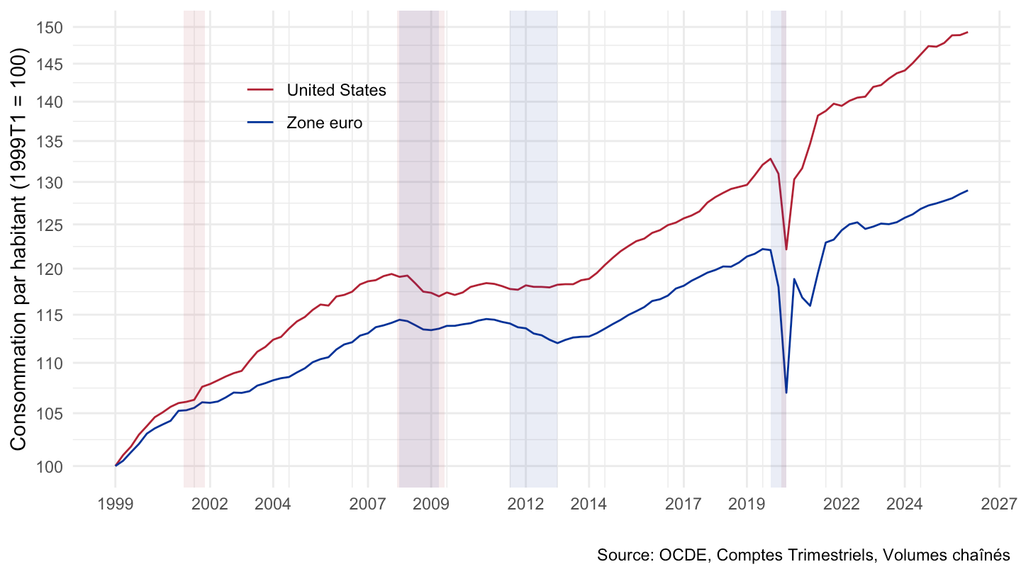
Code
save(plot, file = "QNA_EXPENDITURE_NATIO_CURR_files/figure-html/USA-EA-1999-percapita-1.RData")U.S., Europe, France, Germany
B1GQ - GDP
1995-
Code
QNA_EXPENDITURE_NATIO_CURR %>%
  filter(REF_AREA %in% c("USA", "EA", "FRA", "DEU"),
         FREQ == "Q",
         TRANSACTION == "B1GQ",
         PRICE_BASE == "L",
         ADJUSTMENT == "Y",
         SECTOR == "S1") %>%
  quarter_to_date %>%
  arrange(desc(date)) %>%

  filter(date >= as.Date("1995-01-01")) %>%
  mutate(Ref_area = ifelse(REF_AREA == "EA", "Europe", Ref_area)) %>%
  group_by(Ref_area) %>%
  arrange(date) %>%
  mutate(obsValue = 100 * obsValue / obsValue[1]) %>%
  left_join(colors, by = c("Ref_area" = "country")) %>%
  mutate(color = ifelse(Ref_area != "DEU", color2, color)) %>%
  ggplot(.) + theme_minimal() + xlab("") + ylab("") +
  geom_line(aes(x = date, y = obsValue, color = color)) + add_4flags +
  scale_color_identity() +
  scale_x_date(breaks = c(seq(1995, 2100, 5)) %>% paste0("-01-01") %>% as.Date,
               labels = date_format("%Y")) +
  theme(legend.position = "none") +
  scale_y_log10(breaks = seq(50, 200, 5)) +
  geom_label_repel(data = . %>% filter(date == max(date)),
             aes(x = date, y = obsValue, label = round(obsValue, 1), color = color))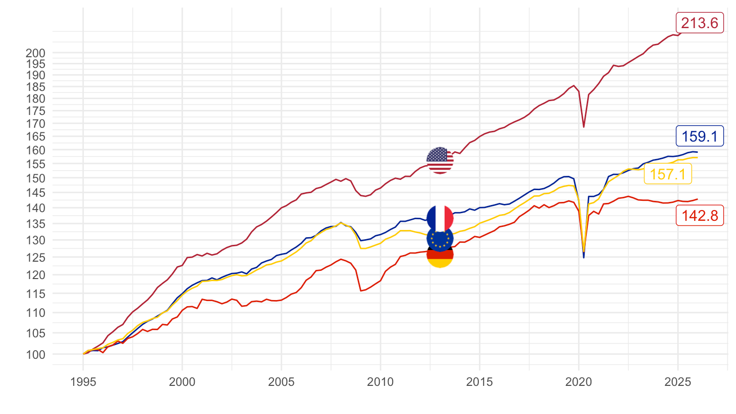
1999-
Total
Code
QNA_EXPENDITURE_NATIO_CURR %>%
  filter(REF_AREA %in% c("USA", "EA", "FRA", "DEU"),
         FREQ == "Q",
         TRANSACTION == "B1GQ",
         PRICE_BASE == "L",
         ADJUSTMENT == "Y",
         SECTOR == "S1") %>%
  quarter_to_date %>%

  filter(date >= as.Date("1999-01-01")) %>%
  mutate(Ref_area = ifelse(REF_AREA == "EA", "Europe", Ref_area)) %>%
  group_by(Ref_area) %>%
  arrange(date) %>%
  mutate(obsValue = 100 * obsValue / obsValue[1]) %>%
  left_join(colors, by = c("Ref_area" = "country")) %>%
  mutate(color = ifelse(Ref_area != "DEU", color2, color)) %>%
  ggplot(.) + theme_minimal() + xlab("") + ylab("") +
  geom_line(aes(x = date, y = obsValue, color = color)) + add_4flags +
  scale_color_identity() +
  scale_x_date(breaks = c(seq(1999, 2100, 5), seq(1997, 2100, 5)) %>% paste0("-01-01") %>% as.Date,
               labels = date_format("%Y")) +
  theme(legend.position = "none") +
  scale_y_log10(breaks = seq(50, 200, 5)) +
  geom_label_repel(data = . %>% filter(date == max(date)),
             aes(x = date, y = obsValue, label = round(obsValue, 1), color = color))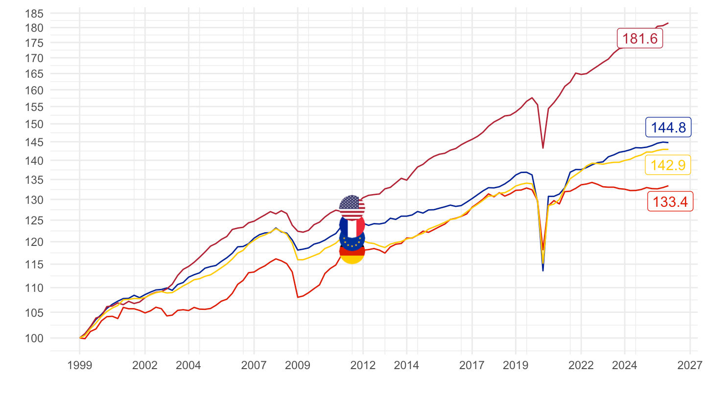
Per Capita
Code
QNA_EXPENDITURE_NATIO_CURR %>%
  filter(REF_AREA %in% c("USA", "EA", "FRA", "DEU"),
         FREQ == "Q",
         TRANSACTION == "B1GQ",
         # L = Chain linked volume
         PRICE_BASE == "L",
         ADJUSTMENT == "Y",
         SECTOR == "S1") %>%
  left_join(QNA_POP_EMPNC_extract, by = c("obsTime", "REF_AREA", "Ref_area")) %>%
  mutate(obsValue = obsValue/population) %>%
  quarter_to_date %>%


  filter(date >= as.Date("1999-01-01")) %>%
  mutate(Ref_area = ifelse(REF_AREA == "EA", "Europe", Ref_area)) %>%
  group_by(Ref_area) %>%
  arrange(date) %>%
  mutate(obsValue = 100 * obsValue / obsValue[1]) %>%
  left_join(colors, by = c("Ref_area" = "country")) %>%
  mutate(color = ifelse(Ref_area != "DEU", color2, color)) %>%
  ggplot(.) + theme_minimal() + xlab("") + ylab("") +
  geom_line(aes(x = date, y = obsValue, color = color)) + add_4flags +
  scale_color_identity() +
  scale_x_date(breaks = c(seq(1999, 2100, 5), seq(1997, 2100, 5)) %>% paste0("-01-01") %>% as.Date,
               labels = date_format("%Y")) +
  theme(legend.position = "none") +
  scale_y_log10(breaks = seq(50, 200, 5)) +
  geom_label_repel(data = . %>% filter(date == max(date)),
             aes(x = date, y = obsValue, label = round(obsValue, 1), color = color))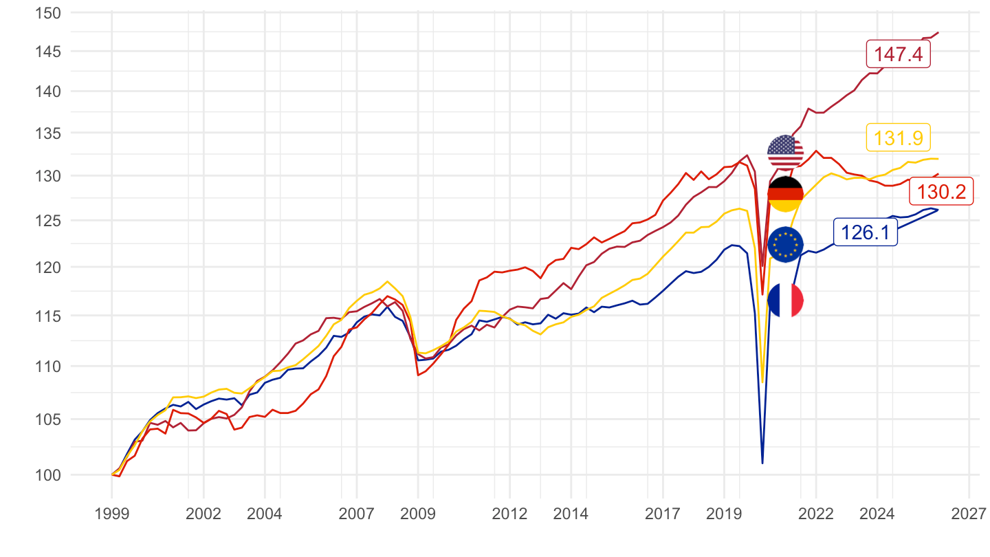
P51G - Gross fixed capital formation
1995-
Code
QNA_EXPENDITURE_NATIO_CURR %>%
  filter(REF_AREA %in% c("USA", "EA", "FRA", "DEU"),
         FREQ == "Q",
         TRANSACTION == "P51G",
         PRICE_BASE == "L",
         ADJUSTMENT == "Y",
         SECTOR == "S1") %>%
  quarter_to_date %>%
  arrange(desc(date)) %>%


  filter(date >= as.Date("1995-01-01")) %>%
  mutate(Ref_area = ifelse(REF_AREA == "EA", "Europe", Ref_area)) %>%
  group_by(Ref_area) %>%
  arrange(date) %>%
  mutate(obsValue = 100 * obsValue / obsValue[1]) %>%
  left_join(colors, by = c("Ref_area" = "country")) %>%
  mutate(color = ifelse(Ref_area != "DEU", color2, color)) %>%
  ggplot(.) + theme_minimal() + xlab("") + ylab("") +
  geom_line(aes(x = date, y = obsValue, color = color)) + add_4flags +
  scale_color_identity() +
  scale_x_date(breaks = c(seq(1995, 2100, 5)) %>% paste0("-01-01") %>% as.Date,
               labels = date_format("%Y")) +
  theme(legend.position = "none") +
  scale_y_log10(breaks = seq(50, 500, 5)) +
  geom_label_repel(data = . %>% filter(date == max(date)),
             aes(x = date, y = obsValue, label = round(obsValue, 1), color = color))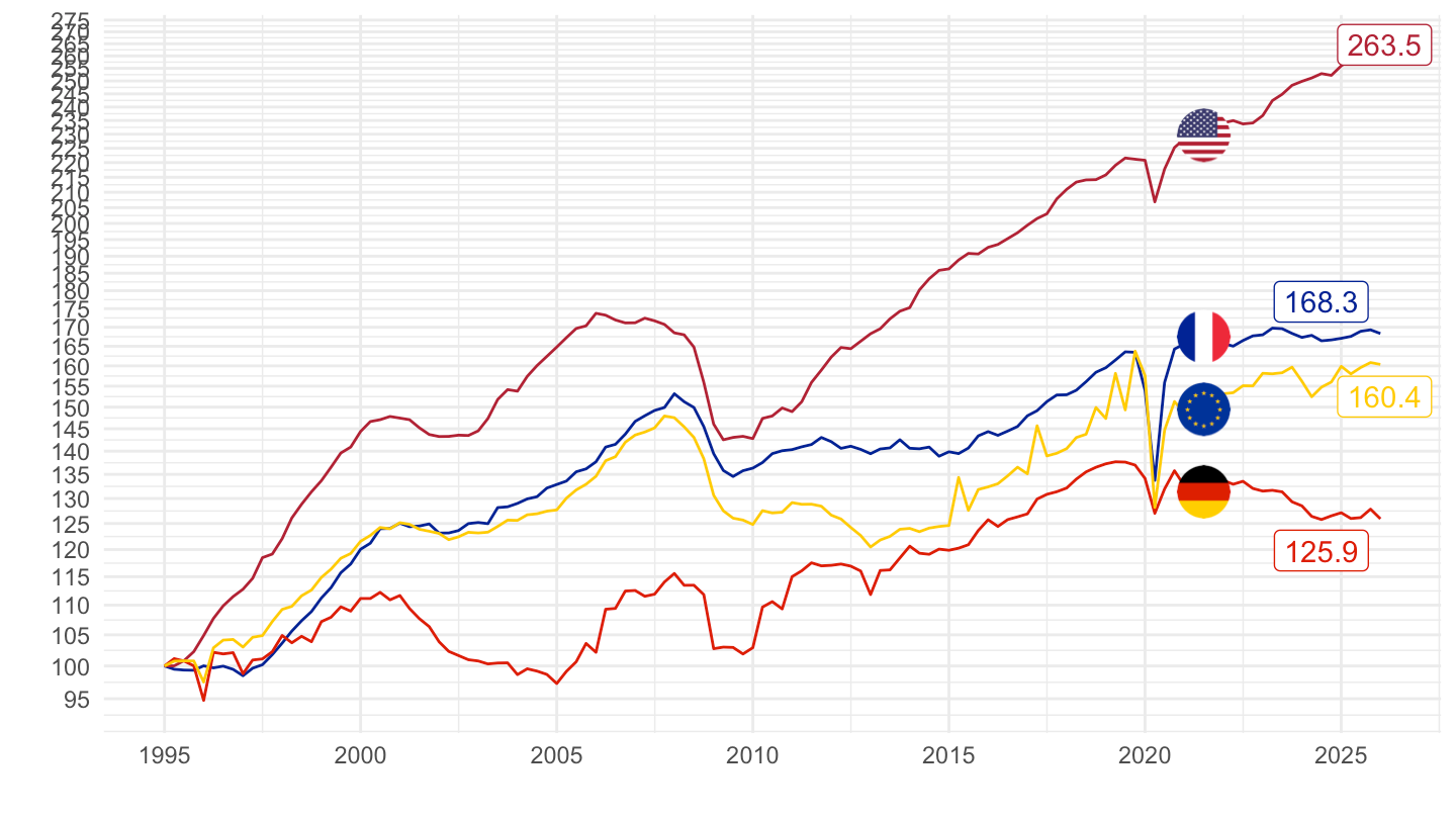
1999-
Total
Code
QNA_EXPENDITURE_NATIO_CURR %>%
  filter(REF_AREA %in% c("USA", "EA", "FRA", "DEU"),
         FREQ == "Q",
         TRANSACTION == "P51G",
         PRICE_BASE == "L",
         ADJUSTMENT == "Y",
         SECTOR == "S1") %>%
  quarter_to_date %>%


  filter(date >= as.Date("1999-01-01")) %>%
  mutate(Ref_area = ifelse(REF_AREA == "EA", "Europe", Ref_area)) %>%
  group_by(Ref_area) %>%
  arrange(date) %>%
  mutate(obsValue = 100 * obsValue / obsValue[1]) %>%
  left_join(colors, by = c("Ref_area" = "country")) %>%
  mutate(color = ifelse(Ref_area != "DEU", color2, color)) %>%
  ggplot(.) + theme_minimal() + xlab("") + ylab("") +
  geom_line(aes(x = date, y = obsValue, color = color)) + add_4flags +
  scale_color_identity() +
  scale_x_date(breaks = c(seq(1999, 2100, 5), seq(1997, 2100, 5)) %>% paste0("-01-01") %>% as.Date,
               labels = date_format("%Y")) +
  theme(legend.position = "none") +
  scale_y_log10(breaks = seq(50, 200, 5)) +
  geom_label_repel(data = . %>% filter(date == max(date)),
             aes(x = date, y = obsValue, label = round(obsValue, 1), color = color))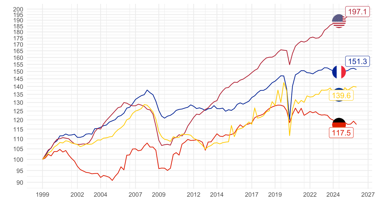
Per Capita
Code
QNA_EXPENDITURE_NATIO_CURR %>%
  filter(REF_AREA %in% c("USA", "EA", "FRA", "DEU"),
         FREQ == "Q",
         TRANSACTION == "P51G",
         # L = Chain linked volume
         PRICE_BASE == "L",
         ADJUSTMENT == "Y",
         SECTOR == "S1") %>%
  left_join(QNA_POP_EMPNC_extract, by = c("obsTime", "REF_AREA", "Ref_area")) %>%
  mutate(obsValue = obsValue/population) %>%
  quarter_to_date %>%


  filter(date >= as.Date("1999-01-01")) %>%
  mutate(Ref_area = ifelse(REF_AREA == "EA", "Europe", Ref_area)) %>%
  group_by(Ref_area) %>%
  arrange(date) %>%
  mutate(obsValue = 100 * obsValue / obsValue[1]) %>%
  left_join(colors, by = c("Ref_area" = "country")) %>%
  mutate(color = ifelse(Ref_area != "DEU", color2, color)) %>%
  ggplot(.) + theme_minimal() + xlab("") + ylab("") +
  geom_line(aes(x = date, y = obsValue, color = color)) + add_4flags +
  scale_color_identity() +
  scale_x_date(breaks = c(seq(1999, 2100, 5), seq(1997, 2100, 5)) %>% paste0("-01-01") %>% as.Date,
               labels = date_format("%Y")) +
  theme(legend.position = "none") +
  scale_y_log10(breaks = seq(50, 200, 5)) +
  geom_label_repel(data = . %>% filter(date == max(date)),
             aes(x = date, y = obsValue, label = round(obsValue, 1), color = color))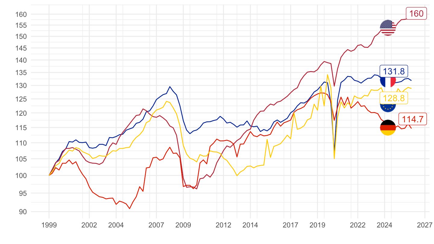
P3 - Final consumption expenditure
All
Code
QNA_EXPENDITURE_NATIO_CURR %>%
  filter(REF_AREA %in% c("USA", "EA", "FRA", "DEU"),
         FREQ == "Q",
         TRANSACTION == "P3",
         PRICE_BASE == "L",
         ADJUSTMENT == "Y",
         SECTOR == "S1") %>%
  quarter_to_date %>%
  arrange(desc(date)) %>%


  mutate(Ref_area = ifelse(REF_AREA == "EA", "Europe", Ref_area)) %>%
  group_by(Ref_area) %>%
  arrange(date) %>%
  mutate(obsValue = 100 * obsValue / obsValue[1]) %>%
  left_join(colors, by = c("Ref_area" = "country")) %>%
  mutate(color = ifelse(Ref_area != "DEU", color2, color)) %>%
  ggplot(.) + theme_minimal() + xlab("") + ylab("") +
  geom_line(aes(x = date, y = obsValue, color = color)) + add_4flags +
  scale_color_identity() +
  scale_x_date(breaks = c(seq(1900, 2100, 5)) %>% paste0("-01-01") %>% as.Date,
               labels = date_format("%Y")) +
  theme(legend.position = "none") +
  scale_y_log10(breaks = seq(20, 600, 20))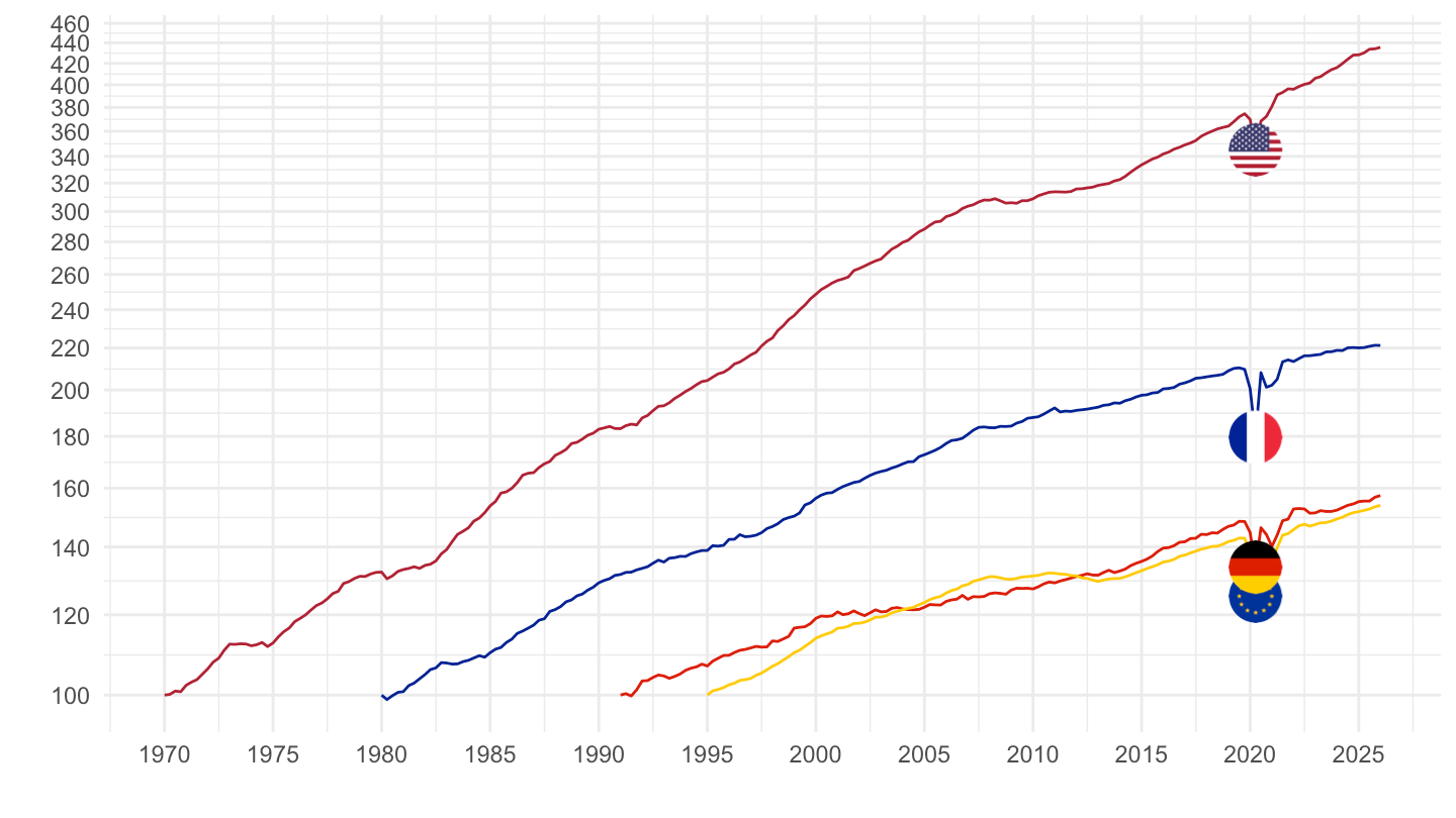
1995-
Code
QNA_EXPENDITURE_NATIO_CURR %>%
  filter(REF_AREA %in% c("USA", "EA", "FRA", "DEU"),
         FREQ == "Q",
         TRANSACTION == "P3",
         PRICE_BASE == "L",
         ADJUSTMENT == "Y",
         SECTOR == "S1") %>%
  quarter_to_date %>%
  arrange(desc(date)) %>%


  filter(date >= as.Date("1995-01-01")) %>%
  mutate(Ref_area = ifelse(REF_AREA == "EA", "Europe", Ref_area)) %>%
  group_by(Ref_area) %>%
  arrange(date) %>%
  mutate(obsValue = 100 * obsValue / obsValue[1]) %>%
  left_join(colors, by = c("Ref_area" = "country")) %>%
  mutate(color = ifelse(Ref_area != "DEU", color2, color)) %>%
  ggplot(.) + theme_minimal() + xlab("") + ylab("") +
  geom_line(aes(x = date, y = obsValue, color = color)) + add_4flags +
  scale_color_identity() +
  scale_x_date(breaks = c(seq(1995, 2100, 5)) %>% paste0("-01-01") %>% as.Date,
               labels = date_format("%Y")) +
  theme(legend.position = "none") +
  scale_y_log10(breaks = seq(50, 200, 5)) +
  geom_label_repel(data = . %>% filter(date == max(date)),
             aes(x = date, y = obsValue, label = round(obsValue, 1), color = color))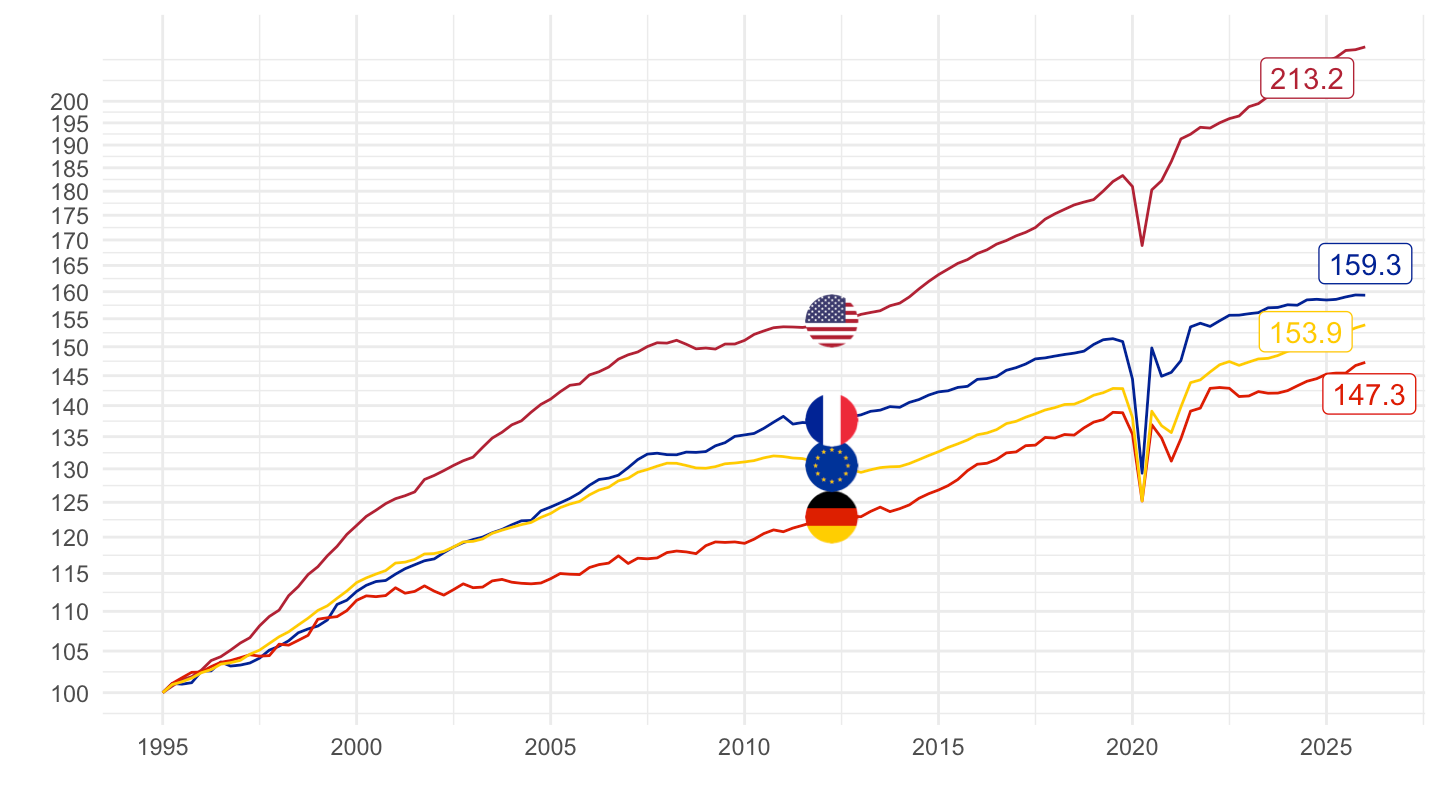
1999-
Total
Code
QNA_EXPENDITURE_NATIO_CURR %>%
  filter(REF_AREA %in% c("USA", "EA", "FRA", "DEU"),
         FREQ == "Q",
         TRANSACTION == "P3",
         # L = Chain linked volume
         PRICE_BASE == "L",
         ADJUSTMENT == "Y",
         SECTOR == "S1") %>%
  quarter_to_date %>%


  filter(date >= as.Date("1999-01-01")) %>%
  mutate(Ref_area = ifelse(REF_AREA == "EA", "Europe", Ref_area)) %>%
  group_by(Ref_area) %>%
  arrange(date) %>%
  mutate(obsValue = 100 * obsValue / obsValue[1]) %>%
  left_join(colors, by = c("Ref_area" = "country")) %>%
  mutate(color = ifelse(Ref_area != "DEU", color2, color)) %>%
  ggplot(.) + theme_minimal() + xlab("") + ylab("") +
  geom_line(aes(x = date, y = obsValue, color = color)) + add_4flags +
  scale_color_identity() +
  scale_x_date(breaks = c(seq(1999, 2100, 5), seq(1997, 2100, 5)) %>% paste0("-01-01") %>% as.Date,
               labels = date_format("%Y")) +
  theme(legend.position = c(0.26, 0.8),
        legend.title = element_blank()) +
  scale_y_log10(breaks = seq(50, 200, 5)) +
  geom_label_repel(data = . %>% filter(date == max(date)),
             aes(x = date, y = obsValue, label = round(obsValue, 1), color = color))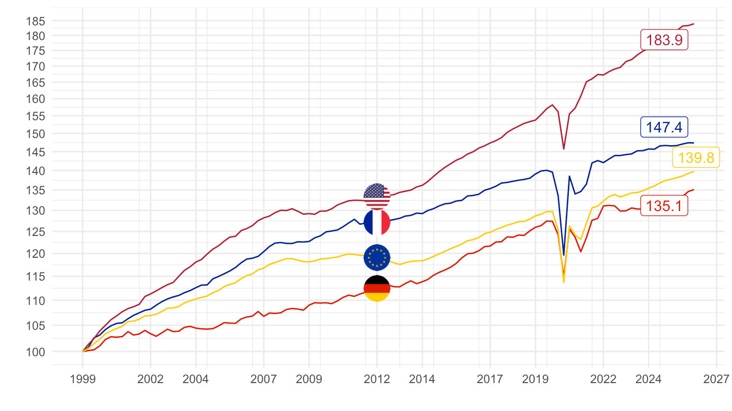
Per Capita
Code
plot <- QNA_EXPENDITURE_NATIO_CURR %>%
  filter(REF_AREA %in% c("USA", "EA", "FRA", "DEU"),
         FREQ == "Q",
         TRANSACTION == "P3",
         # L = Chain linked volume
         PRICE_BASE == "L",
         ADJUSTMENT == "Y",
         SECTOR == "S1") %>%
  left_join(QNA_POP_EMPNC_extract, by = c("obsTime", "REF_AREA", "Ref_area")) %>%
  mutate(obsValue = obsValue/population) %>%
  quarter_to_date %>%

  filter(date >= as.Date("1999-01-01")) %>%
  mutate(Ref_area = ifelse(REF_AREA == "EA", "Zone euro", Ref_area)) %>%
  group_by(Ref_area) %>%
  arrange(date) %>%
  mutate(obsValue = 100 * obsValue / obsValue[1]) %>%
  ggplot(.) + theme_minimal() + xlab("") + ylab("Consommation par habitant (1999T1 = 100)") +
  geom_line(aes(x = date, y = obsValue, color = Ref_area)) +
  scale_color_manual(values = c("#000000", "#B22234", "#808080", "#003399")) +
  scale_x_date(breaks = c(seq(1999, 2100, 5), seq(1997, 2100, 5)) %>% paste0("-01-01") %>% as.Date,
               labels = date_format("%Y")) +
  theme(legend.position = c(0.26, 0.8),
        legend.title = element_blank()) +
  scale_y_log10(breaks = seq(50, 200, 5))  +
  geom_rect(data = nber_recessions %>%
              filter(Peak > as.Date("1999-01-01")),
            aes(xmin = Peak, xmax = Trough, ymin = 0, ymax = +Inf),
            fill = '#B22234', alpha = 0.1)  +
  geom_rect(data = cepr_recessions %>%
              filter(Peak > as.Date("1999-01-01")),
            aes(xmin = Peak, xmax = Trough, ymin = 0, ymax = +Inf),
            fill = '#003399', alpha = 0.1)  +
  labs(caption = "Source: OCDE, Comptes Trimestriels, Volumes chaînés")


save(plot, file = "QNA_EXPENDITURE_NATIO_CURR_files/figure-html/USA-EA-FRA-DEU-1999-percapita-1.RData")

plot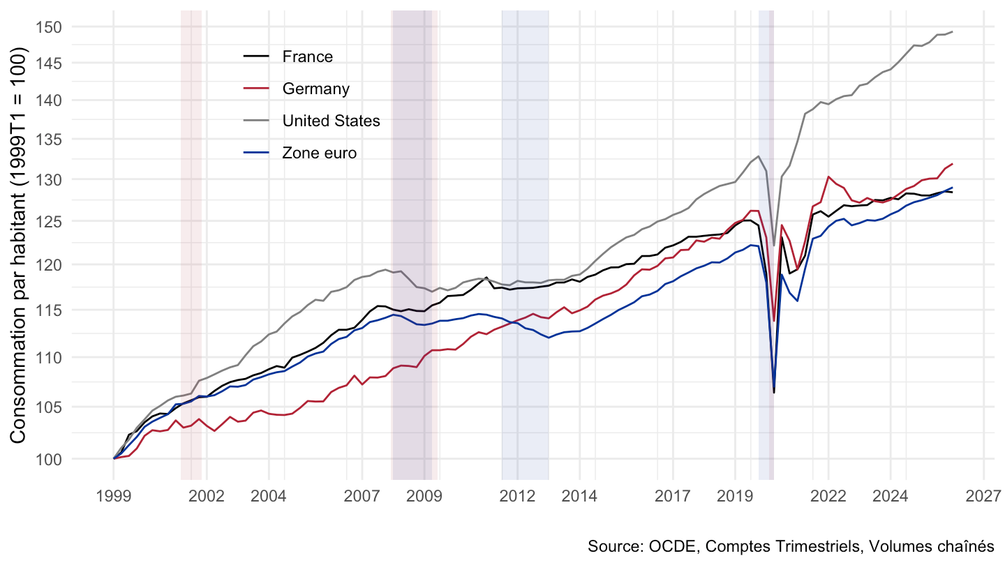
P31 - Individual consumption expenditure
Code
QNA_EXPENDITURE_NATIO_CURR %>%
  filter(REF_AREA %in% c("USA", "EA", "FRA", "DEU"),
         FREQ == "Q",
         TRANSACTION == "P31",
         # L = Chain linked volume
         PRICE_BASE == "L",
         ADJUSTMENT == "Y") %>%
  left_join(QNA_POP_EMPNC_extract, by = c("obsTime", "REF_AREA", "Ref_area")) %>%
  mutate(obsValue = obsValue/population) %>%
  quarter_to_date %>%


  filter(date >= as.Date("1999-01-01")) %>%
  mutate(Ref_area = ifelse(REF_AREA == "EA", "Europe", Ref_area)) %>%
  group_by(Ref_area) %>%
  arrange(date) %>%
  mutate(obsValue = 100 * obsValue / obsValue[1]) %>%
  left_join(colors, by = c("Ref_area" = "country")) %>%
  mutate(color = ifelse(Ref_area != "DEU", color2, color)) %>%
  ggplot(.) + theme_minimal() + xlab("") + ylab("") +
  geom_line(aes(x = date, y = obsValue, color = color)) + add_3flags +
  scale_color_identity() +
  scale_x_date(breaks = c(seq(1999, 2100, 5), seq(1997, 2100, 5)) %>% paste0("-01-01") %>% as.Date,
               labels = date_format("%Y")) +
  theme(legend.position = "none") +
  scale_y_log10(breaks = seq(50, 200, 5)) +
  geom_label_repel(data = . %>% filter(date == max(date)),
             aes(x = date, y = obsValue, label = round(obsValue, 1), color = color))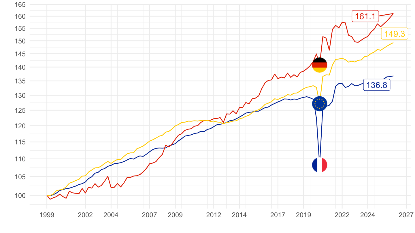
P32 - Collective consumption expenditure
Code
QNA_EXPENDITURE_NATIO_CURR %>%
  filter(REF_AREA %in% c("USA", "EA", "FRA", "DEU"),
         FREQ == "Q",
         TRANSACTION == "P32",
         # L = Chain linked volume
         PRICE_BASE == "L",
         ADJUSTMENT == "Y") %>%
  left_join(QNA_POP_EMPNC_extract, by = c("obsTime", "REF_AREA", "Ref_area")) %>%
  mutate(obsValue = obsValue/population) %>%
  quarter_to_date %>%


  filter(date >= as.Date("1999-01-01")) %>%
  mutate(Ref_area = ifelse(REF_AREA == "EA", "Europe", Ref_area)) %>%
  group_by(Ref_area) %>%
  arrange(date) %>%
  mutate(obsValue = 100 * obsValue / obsValue[1]) %>%
  left_join(colors, by = c("Ref_area" = "country")) %>%
  mutate(color = ifelse(Ref_area != "DEU", color2, color)) %>%
  ggplot(.) + theme_minimal() + xlab("") + ylab("") +
  geom_line(aes(x = date, y = obsValue, color = color)) + add_3flags +
  scale_color_identity() +
  scale_x_date(breaks = c(seq(1999, 2100, 5), seq(1997, 2100, 5)) %>% paste0("-01-01") %>% as.Date,
               labels = date_format("%Y")) +
  theme(legend.position = "none") +
  scale_y_log10(breaks = seq(50, 200, 5)) +
  geom_label_repel(data = . %>% filter(date == max(date)),
             aes(x = date, y = obsValue, label = round(obsValue, 1), color = color))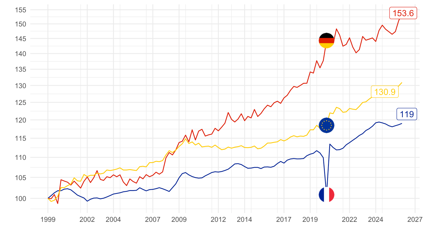
P41 - Actual individual consumption
Code
QNA_EXPENDITURE_NATIO_CURR %>%
  filter(REF_AREA %in% c("USA", "EA", "FRA", "DEU"),
         FREQ == "Q",
         TRANSACTION == "P41",
         # L = Chain linked volume
         PRICE_BASE == "L",
         ADJUSTMENT == "Y") %>%
     left_join(QNA_POP_EMPNC_extract, by = c("obsTime", "REF_AREA", "Ref_area")) %>%
  mutate(obsValue = obsValue/population) %>%
  quarter_to_date %>%


  filter(date >= as.Date("1999-01-01")) %>%
  mutate(Ref_area = ifelse(REF_AREA == "EA", "Europe", Ref_area)) %>%
  group_by(Ref_area) %>%
  arrange(date) %>%
  mutate(obsValue = 100 * obsValue / obsValue[1]) %>%
  left_join(colors, by = c("Ref_area" = "country")) %>%
  mutate(color = ifelse(Ref_area != "DEU", color2, color)) %>%
  ggplot(.) + theme_minimal() + xlab("") + ylab("") +
  geom_line(aes(x = date, y = obsValue, color = color)) + add_2flags +
  scale_color_identity() +
  scale_x_date(breaks = c(seq(1999, 2100, 5), seq(1997, 2100, 5)) %>% paste0("-01-01") %>% as.Date,
               labels = date_format("%Y")) +
  theme(legend.position = "none") +
  scale_y_log10(breaks = seq(50, 200, 5)) +
  geom_label_repel(data = . %>% filter(date == max(date)),
             aes(x = date, y = obsValue, label = round(obsValue, 1), color = color))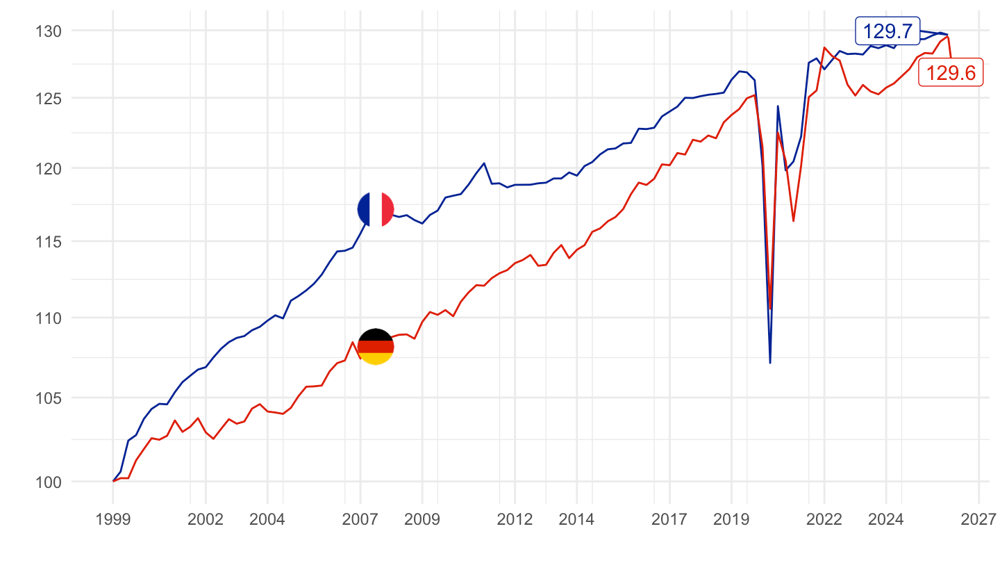
P3T5 - Domestic demand
Code
QNA_EXPENDITURE_NATIO_CURR %>%
  filter(REF_AREA %in% c("USA", "EA", "FRA", "DEU"),
         FREQ == "Q",
         TRANSACTION == "P3T5",
         # L = Chain linked volume
         PRICE_BASE == "L",
         ADJUSTMENT == "Y") %>%
     left_join(QNA_POP_EMPNC_extract, by = c("obsTime", "REF_AREA", "Ref_area")) %>%
  mutate(obsValue = obsValue/population) %>%
  quarter_to_date %>%


  filter(date >= as.Date("1999-01-01")) %>%
  mutate(Ref_area = ifelse(REF_AREA == "EA", "Europe", Ref_area)) %>%
  group_by(Ref_area) %>%
  arrange(date) %>%
  mutate(obsValue = 100 * obsValue / obsValue[1]) %>%
  left_join(colors, by = c("Ref_area" = "country")) %>%
  mutate(color = ifelse(Ref_area != "DEU", color2, color)) %>%
  ggplot(.) + theme_minimal() + xlab("") + ylab("") +
  geom_line(aes(x = date, y = obsValue, color = color)) + add_3flags +
  scale_color_identity() +
  scale_x_date(breaks = c(seq(1999, 2100, 5), seq(1997, 2100, 5)) %>% paste0("-01-01") %>% as.Date,
               labels = date_format("%Y")) +
  theme(legend.position = "none") +
  scale_y_log10(breaks = seq(50, 200, 5)) +
  geom_label_repel(data = . %>% filter(date == max(date)),
             aes(x = date, y = obsValue, label = round(obsValue, 1), color = color))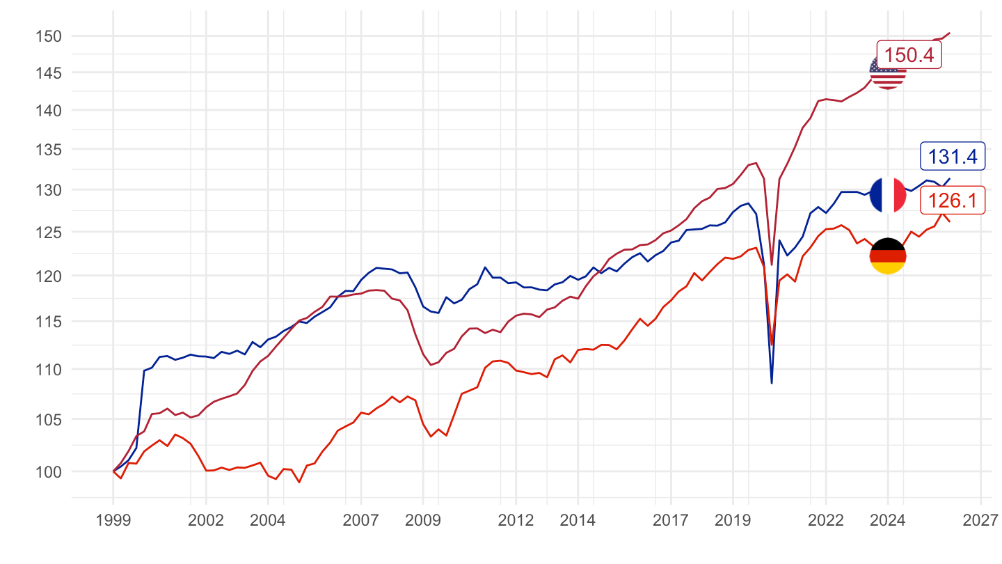
Net exports
Eurozone, US, France, Germany
Tous
Code
QNA_EXPENDITURE_NATIO_CURR %>%
  filter(REF_AREA %in% c("EA", "USA", "DEU", "FRA"),
         FREQ == "Q",
         TRANSACTION %in% c("B11", "B1GQ"),
         # L = Chain linked volume
         PRICE_BASE == "V",
         ADJUSTMENT == "Y") %>%

  mutate(Ref_area = ifelse(REF_AREA == "EA", "Europe", Ref_area)) %>%
  group_by(Ref_area) %>%
  select_if(~ n_distinct(.) > 1) %>%
  select(-OBS_STATUS) %>%
  spread(TRANSACTION, obsValue) %>%
  quarter_to_date() %>%
  filter(date >= as.Date("1970-01-01")) %>%
  transmute(date, Ref_area, obsValue = B11/B1GQ) %>%
  left_join(colors, by = c("Ref_area" = "country")) %>%
  ggplot + geom_line(aes(x = date, y = obsValue, color = color)) +
  theme_minimal() + xlab("") + ylab("") + scale_color_identity() + add_4flags +
  scale_x_date(breaks = c(seq(1970, 2100, 5)) %>% paste0("-01-01") %>% as.Date,
               labels = date_format("%Y")) +
  scale_y_continuous(breaks = 0.01*seq(-100, 100, 1),
                labels = percent_format(acc = 1)) +
  theme(legend.position = c(0.2, 0.8),
        legend.title = element_blank()) +
  geom_hline(yintercept = 0, linetype = "dashed")
1990-
Code
QNA_EXPENDITURE_NATIO_CURR %>%
  filter(REF_AREA %in% c("EA", "USA", "DEU", "FRA"),
         FREQ == "Q",
         TRANSACTION %in% c("B11", "B1GQ"),
         # L = Chain linked volume
         PRICE_BASE == "V",
         ADJUSTMENT == "Y") %>%


  mutate(Ref_area = ifelse(REF_AREA == "EA", "Europe", Ref_area)) %>%
  group_by(Ref_area) %>%
  select_if(~ n_distinct(.) > 1) %>%
  select(-OBS_STATUS) %>%
  spread(TRANSACTION, obsValue) %>%
  quarter_to_date() %>%
  filter(date >= as.Date("1990-01-01")) %>%
  transmute(date, Ref_area, obsValue = B11/B1GQ) %>%
  left_join(colors, by = c("Ref_area" = "country")) %>%
  ggplot + geom_line(aes(x = date, y = obsValue, color = color)) +
  theme_minimal() + xlab("") + ylab("") + scale_color_identity() + add_4flags +
  scale_x_date(breaks = c(seq(1970, 2100, 5)) %>% paste0("-01-01") %>% as.Date,
               labels = date_format("%Y")) +
  scale_y_continuous(breaks = 0.01*seq(-100, 100, 1),
                labels = percent_format(acc = 1)) +
  theme(legend.position = c(0.2, 0.8),
        legend.title = element_blank()) +
  geom_hline(yintercept = 0, linetype = "dashed")
Eurozone, US
Tous
Code
QNA_EXPENDITURE_NATIO_CURR %>%
  filter(REF_AREA %in% c("EA", "USA"),
         FREQ == "Q",
         TRANSACTION %in% c("B11", "B1GQ"),
         # L = Chain linked volume
         PRICE_BASE == "V",
         ADJUSTMENT == "Y") %>%

  mutate(Ref_area = ifelse(REF_AREA == "EA", "Europe", Ref_area)) %>%
  group_by(Ref_area) %>%
  select_if(~ n_distinct(.) > 1) %>%
  spread(TRANSACTION, obsValue) %>%
  quarter_to_date() %>%
  transmute(date, REF_AREA, Ref_area, obsValue = B11/B1GQ) %>%
  left_join(colors, by = c("Ref_area" = "country")) %>%
  mutate(color = ifelse(REF_AREA == "USA", color2, color)) %>%
  ggplot + geom_line(aes(x = date, y = obsValue, color = color)) +
  theme_minimal() + xlab("") + ylab("") + scale_color_identity() + add_2flags +
  scale_x_date(breaks = c(seq(1920, 2100, 5)) %>% paste0("-01-01") %>% as.Date,
               labels = date_format("%Y")) +
  scale_y_continuous(breaks = 0.01*seq(-100, 100, 1),
                labels = percent_format(acc = 1)) +
  theme(legend.position = c(0.2, 0.8),
        legend.title = element_blank()) +
  geom_hline(yintercept = 0, linetype = "dashed")
1970-
Code
QNA_EXPENDITURE_NATIO_CURR %>%
  filter(REF_AREA %in% c("EA", "USA"),
         FREQ == "Q",
         TRANSACTION %in% c("B11", "B1GQ"),
         # L = Chain linked volume
         PRICE_BASE == "V",
         ADJUSTMENT == "Y") %>%

  mutate(Ref_area = ifelse(REF_AREA == "EA", "Europe", Ref_area)) %>%
  group_by(Ref_area) %>%
  select_if(~ n_distinct(.) > 1) %>%
  spread(TRANSACTION, obsValue) %>%
  quarter_to_date() %>%
  filter(date >= as.Date("1970-01-01")) %>%
  transmute(date, REF_AREA, Ref_area, obsValue = B11/B1GQ) %>%
  left_join(colors, by = c("Ref_area" = "country")) %>%
  mutate(color = ifelse(REF_AREA == "USA", color2, color)) %>%
  ggplot + geom_line(aes(x = date, y = obsValue, color = color)) +
  theme_minimal() + xlab("") + ylab("") + scale_color_identity() + add_2flags +
  scale_x_date(breaks = c(seq(1970, 2100, 5)) %>% paste0("-01-01") %>% as.Date,
               labels = date_format("%Y")) +
  scale_y_continuous(breaks = 0.01*seq(-100, 100, 1),
                labels = percent_format(acc = 1)) +
  theme(legend.position = c(0.2, 0.8),
        legend.title = element_blank()) +
  geom_hline(yintercept = 0, linetype = "dashed")
1990-
Code
QNA_EXPENDITURE_NATIO_CURR %>%
  filter(REF_AREA %in% c("EA", "USA"),
         FREQ == "Q",
         TRANSACTION %in% c("B11", "B1GQ"),
         # L = Chain linked volume
         PRICE_BASE == "V",
         ADJUSTMENT == "Y") %>%

  mutate(Ref_area = ifelse(REF_AREA == "EA", "Europe", Ref_area)) %>%
  group_by(Ref_area) %>%
  select_if(~ n_distinct(.) > 1) %>%
  spread(TRANSACTION, obsValue) %>%
  quarter_to_date() %>%
  filter(date >= as.Date("1995-01-01")) %>%
  transmute(date, REF_AREA, Ref_area, obsValue = B11/B1GQ) %>%
  left_join(colors, by = c("Ref_area" = "country")) %>%
  mutate(color = ifelse(REF_AREA == "USA", color2, color)) %>%
  ggplot + geom_line(aes(x = date, y = obsValue, color = color)) +
  theme_minimal() + xlab("") + ylab("") + scale_color_identity() + add_2flags +
  scale_x_date(breaks = c(seq(1970, 2100, 5)) %>% paste0("-01-01") %>% as.Date,
               labels = date_format("%Y")) +
  scale_y_continuous(breaks = 0.01*seq(-100, 100, 1),
                labels = percent_format(acc = 1)) +
  theme(legend.position = c(0.2, 0.8),
        legend.title = element_blank()) +
  geom_hline(yintercept = 0, linetype = "dashed")
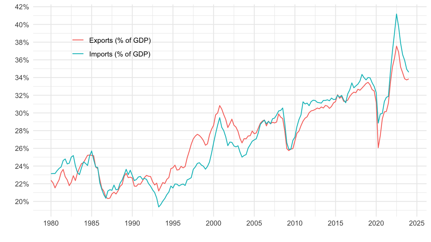
Exports and Imports as a % of GDP
EA 20
Code
QNA_EXPENDITURE_NATIO_CURR %>%
  filter(REF_AREA %in% c("EA"),
         FREQ == "Q",
         TRANSACTION %in% c("P6", "P7", "B1GQ"),
         # L = Chain linked volume
         PRICE_BASE == "L",
         ADJUSTMENT == "Y") %>%
  select_if(~ n_distinct(.) > 1) %>%
  select(-OBS_STATUS) %>%
  spread(TRANSACTION, obsValue) %>%
  quarter_to_date() %>%
  transmute(date, `Exports (% of GDP)` = P6/B1GQ, `Imports (% of GDP)` = P7/B1GQ) %>%
  gather(variable, value, -date) %>%
  ggplot + geom_line(aes(x = date, y = value, color = variable)) +
  theme_minimal() + xlab("") + ylab("") +
  scale_x_date(breaks = c(seq(1999, 2100, 5), seq(1997, 2100, 5)) %>% paste0("-01-01") %>% as.Date,
               labels = date_format("%Y")) +
  scale_y_continuous(breaks = 0.01*seq(-100, 100, 5),
                labels = percent_format(acc = 1)) +
  theme(legend.position = c(0.2, 0.8),
        legend.title = element_blank())
USA
Code
QNA_EXPENDITURE_NATIO_CURR %>%
  filter(REF_AREA %in% c("USA"),
         FREQ == "Q",
         TRANSACTION %in% c("P6", "P7", "B1GQ"),
         # L = Chain linked volume
         PRICE_BASE == "V",
         ADJUSTMENT == "Y") %>%
  select_if(~ n_distinct(.) > 1) %>%
  spread(TRANSACTION, obsValue) %>%
  quarter_to_date() %>%
  transmute(date, `Exports (% of GDP)` = P6/B1GQ, `Imports (% of GDP)` = P7/B1GQ) %>%
  gather(variable, value, -date) %>%
  ggplot + geom_line(aes(x = date, y = value, color = variable)) +
  theme_minimal() + xlab("") + ylab("") +
  scale_x_date(breaks = c(seq(1940, 2100, 5)) %>% paste0("-01-01") %>% as.Date,
               labels = date_format("%Y")) +
  scale_y_continuous(breaks = 0.01*seq(-100, 100, 2),
                labels = percent_format(acc = 1)) +
  theme(legend.position = c(0.2, 0.8),
        legend.title = element_blank())
Germany
Code
QNA_EXPENDITURE_NATIO_CURR %>%
  filter(REF_AREA %in% c("DEU"),
         FREQ == "Q",
         TRANSACTION %in% c("P6", "P7", "B1GQ"),
         # L = Chain linked volume
         PRICE_BASE == "V",
         ADJUSTMENT == "Y") %>%
  select_if(~ n_distinct(.) > 1) %>%
  spread(TRANSACTION, obsValue) %>%
  quarter_to_date() %>%
  transmute(date, `Exports (% of GDP)` = P6/B1GQ, `Imports (% of GDP)` = P7/B1GQ) %>%
  gather(variable, value, -date) %>%
  ggplot + geom_line(aes(x = date, y = value, color = variable)) +
  theme_minimal() + xlab("") + ylab("") +
  scale_x_date(breaks = c(seq(1940, 2100, 5)) %>% paste0("-01-01") %>% as.Date,
               labels = date_format("%Y")) +
  scale_y_continuous(breaks = 0.01*seq(-100, 100, 2),
                labels = percent_format(acc = 1)) +
  theme(legend.position = c(0.2, 0.8),
        legend.title = element_blank())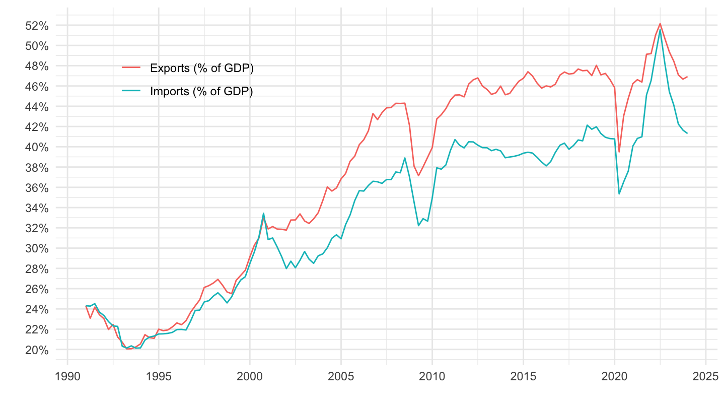
France
Code
QNA_EXPENDITURE_NATIO_CURR %>%
  filter(REF_AREA %in% c("FRA"),
         FREQ == "Q",
         TRANSACTION %in% c("P6", "P7", "B1GQ"),
         # L = Chain linked volume
         PRICE_BASE == "V",
         ADJUSTMENT == "Y") %>%
  select_if(~ n_distinct(.) > 1) %>%
  spread(TRANSACTION, obsValue) %>%
  quarter_to_date() %>%
  transmute(date, `Exports (% of GDP)` = P6/B1GQ, `Imports (% of GDP)` = P7/B1GQ) %>%
  gather(variable, value, -date) %>%
  ggplot + geom_line(aes(x = date, y = value, color = variable)) +
  theme_minimal() + xlab("") + ylab("") +
  scale_x_date(breaks = c(seq(1940, 2100, 5)) %>% paste0("-01-01") %>% as.Date,
               labels = date_format("%Y")) +
  scale_y_continuous(breaks = 0.01*seq(-100, 100, 2),
                labels = percent_format(acc = 1)) +
  theme(legend.position = c(0.2, 0.8),
        legend.title = element_blank())