Population and employment

Data - Eurostat

Author

François Geerolf

Info

Last observation: Quarterly: 2026Q2 (N = 128)

First observation: Quarterly: 1980Q1 (N = 8)

Last data update: 11 aoû 2026, 21:34. Last compile: 12 aoû 2026, 02:16

Structure

Population Table

Code

namq_10_pe |>
  filter(time %in% c("2019Q1", "2009Q1", "1999Q1", "1989Q1"),
         na_item == "POP_NC",
         s_adj %in% c("SCA", "SA"),
         unit == "THS_PER") |>
  select(geo, s_adj, time, values) |>
  mutate(values = round(values/1000, 1)) |>
  
  spread(time, values) |>
  arrange(- `2009Q1`) %>%
  {if (is_html_output()) datatable(., filter = 'top', rownames = F) else .}

Employment Table

Code

namq_10_pe |>
  filter(time %in% c("2019Q1", "2009Q1", "1999Q1", "1989Q1"),
         na_item == "EMP_DC",
         s_adj %in% c("SCA", "SA"),
         unit == "THS_PER") |>
  select(geo, s_adj, time, values) |>
  mutate(values = round(values/1000, 1)) |>
  
  spread(time, values) |>
  arrange(- `2019Q1`) %>%
  {if (is_html_output()) datatable(., filter = 'top', rownames = F) else .}

Eurozone

Last observation

Code

namq_10_pe |>
  filter(na_item == "POP_NC") |>
  filter(time == max(time)) |>
  spread(unit, values) %>%
  select_if(~ n_distinct(.) > 1) |>
  
  select(geo, Geo, everything()) |>
  print_table_conditional()

geo	Geo	Unit	s_adj	S_adj	PCH_PRE_PER	PCH_SM_PER	THS_PER
ES	Spain	Percentage change compared to same period in previous year (based on persons)	NSA	Unadjusted data (i.e. neither seasonally adjusted nor calendar adjusted data)	NA	1.0	NA
NL	Netherlands	Percentage change compared to same period in previous year (based on persons)	NSA	Unadjusted data (i.e. neither seasonally adjusted nor calendar adjusted data)	NA	0.4	NA
ES	Spain	Percentage change compared to same period in previous year (based on persons)	SCA	Seasonally and calendar adjusted data	NA	1.0	NA
NL	Netherlands	Percentage change compared to same period in previous year (based on persons)	SCA	Seasonally and calendar adjusted data	NA	0.4	NA
ES	Spain	Percentage change on previous period (based on persons)	SCA	Seasonally and calendar adjusted data	0.2	NA	NA
NL	Netherlands	Percentage change on previous period (based on persons)	SCA	Seasonally and calendar adjusted data	0.0	NA	NA
ES	Spain	Thousand persons	NSA	Unadjusted data (i.e. neither seasonally adjusted nor calendar adjusted data)	NA	NA	49737.05
NL	Netherlands	Thousand persons	NSA	Unadjusted data (i.e. neither seasonally adjusted nor calendar adjusted data)	NA	NA	18135.00
ES	Spain	Thousand persons	SCA	Seasonally and calendar adjusted data	NA	NA	49737.05
NL	Netherlands	Thousand persons	SCA	Seasonally and calendar adjusted data	NA	NA	18135.00

Previous observation

Code

namq_10_pe |>
  filter(time %in% c("2023Q4", "2023Q3"),
         na_item == "POP_NC",
         geo == "EA20") |>
  spread(time, values) %>%
  select_if(~ n_distinct(.) > 1) |>
  print_table_conditional()

unit	Unit	s_adj	S_adj	2023Q3	2023Q4
PCH_PRE_PER	Percentage change on previous period (based on persons)	SCA	Seasonally and calendar adjusted data	0.1	0.1
PCH_SM_PER	Percentage change compared to same period in previous year (based on persons)	NSA	Unadjusted data (i.e. neither seasonally adjusted nor calendar adjusted data)	0.6	0.5
PCH_SM_PER	Percentage change compared to same period in previous year (based on persons)	SCA	Seasonally and calendar adjusted data	0.6	0.5
THS_PER	Thousand persons	NSA	Unadjusted data (i.e. neither seasonally adjusted nor calendar adjusted data)	349857.2	350399.6
THS_PER	Thousand persons	SCA	Seasonally and calendar adjusted data	349873.7	350366.6

France, Germany, Italy, Europe

Population

All

Code

namq_10_pe |>
  filter(geo %in% c("FR", "DE", "IT", "EA20"),
         unit == "THS_PER",
         s_adj == "NSA",
         na_item == "POP_NC") |>
  
  quarter_to_date() |>
  group_by(geo) |>
  mutate(values = 100*values/values[1]) %>%
  select_if(~ n_distinct(.) > 1) |>
  mutate(Geo = ifelse(geo == "EA20", "Europe", Geo)) |>
  left_join(colors, by = c( "Geo" = "country")) |>
  ggplot() + ylab("Population") + xlab("") + theme_minimal() +
  geom_line(aes(x = date, y = values, color = color)) +
  scale_color_identity() + theme_minimal() + add_flags +
  scale_x_date(breaks = seq(1909, 2100, 5) |> paste0("-01-01") |> as.Date(),
               labels = date_format("%Y")) +
  theme(legend.position = c(0.3, 0.7),
        legend.title = element_blank()) +
  scale_y_log10(breaks = seq(10, 300, 2),
                     labels = dollar_format(accuracy = 1, prefix = "")) +
  geom_label_repel(data = . %>% group_by(Geo) %>% filter(date == max(date)), aes(x = date, y = values, label = round(values, 1), color = color), show.legend = F)

1999-

Code

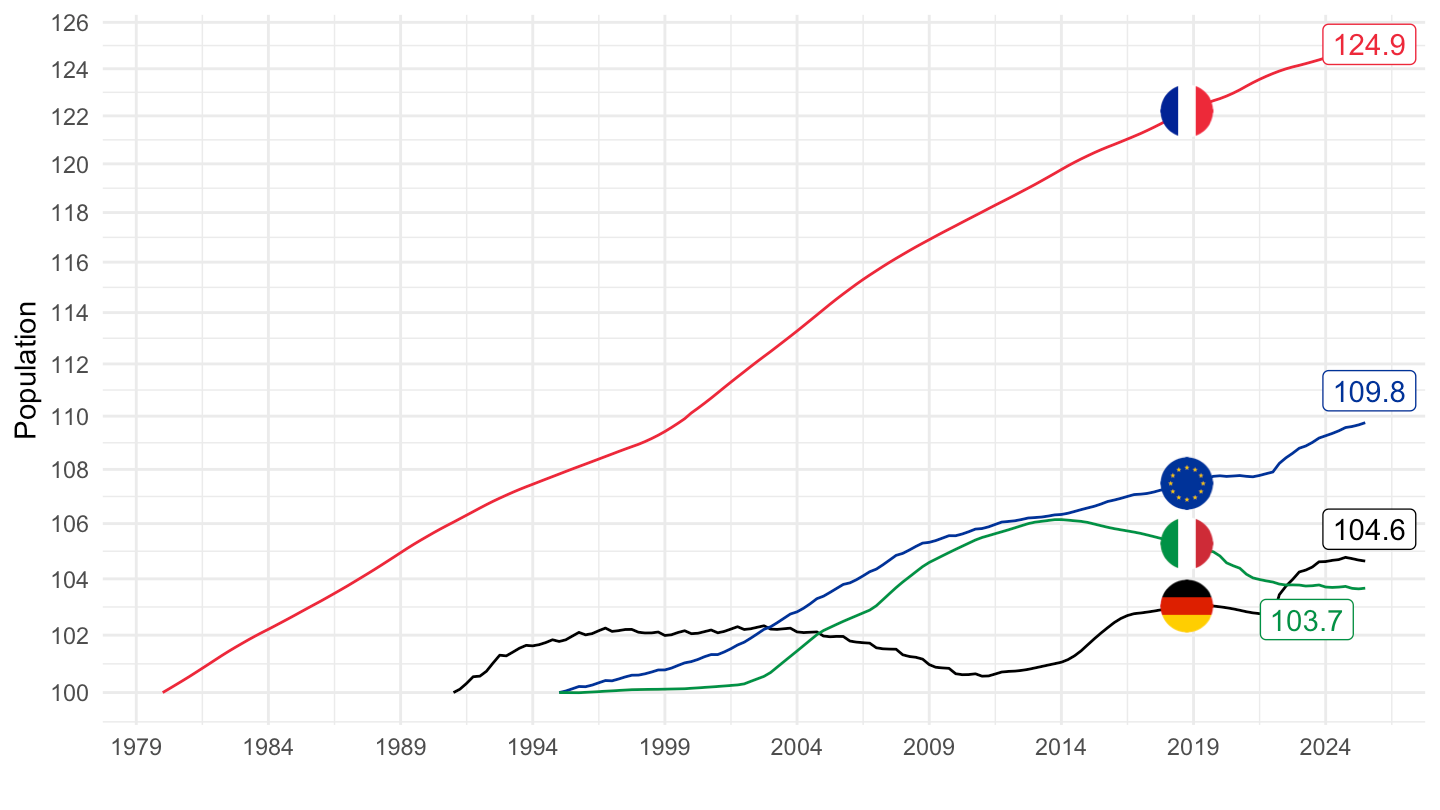
namq_10_pe |>
  filter(geo %in% c("FR", "DE", "IT", "EA20"),
         unit == "THS_PER",
         s_adj == "NSA",
         na_item == "POP_NC") |>
  
  quarter_to_date() |>
  filter(date >= as.Date("1999-01-01")) |>
  group_by(geo) |>
  mutate(values = 100*values/values[1]) %>%
  select_if(~ n_distinct(.) > 1) |>
  mutate(Geo = ifelse(geo == "EA20", "Europe", Geo)) |>
  left_join(colors, by = c( "Geo" = "country")) |>
  ggplot() + ylab("Population") + xlab("") + theme_minimal() +
  geom_line(aes(x = date, y = values, color = color)) +
  scale_color_identity() + theme_minimal() + add_flags +
  scale_x_date(breaks = seq(1909, 2100, 5) |> paste0("-01-01") |> as.Date(),
               labels = date_format("%Y")) +
  theme(legend.position = c(0.3, 0.7),
        legend.title = element_blank()) +
  scale_y_log10(breaks = seq(10, 300, 2),
                     labels = dollar_format(accuracy = 1, prefix = "")) +
  geom_label_repel(data = . %>% group_by(Geo) %>% filter(date == max(date)), aes(x = date, y = values, label = round(values, 1), color = color), show.legend = F)

2001-2021

Code

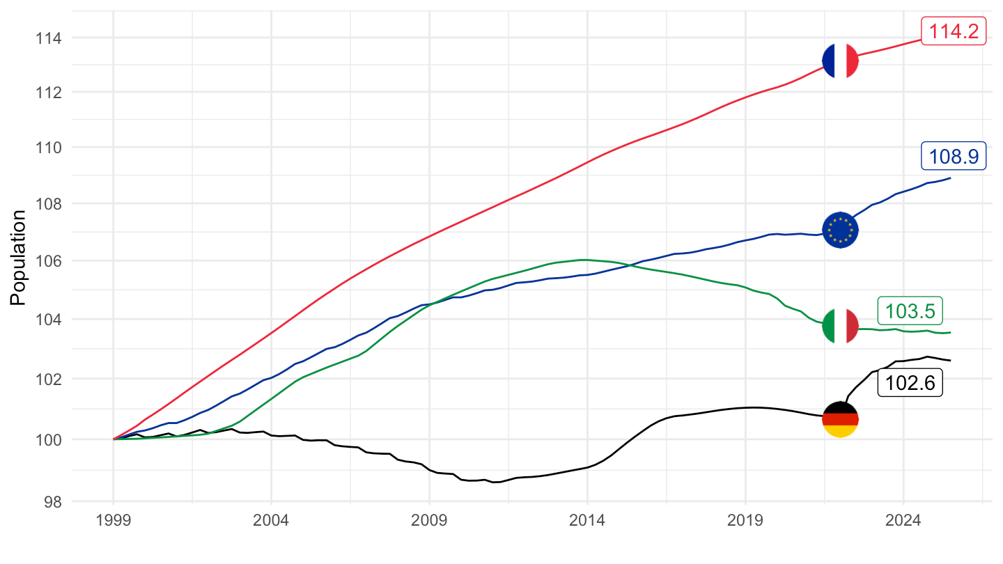
namq_10_pe |>
  filter(geo %in% c("FR", "DE", "IT", "EA20"),
         unit == "THS_PER",
         s_adj == "NSA",
         na_item == "POP_NC") |>
  
  quarter_to_date() |>
  filter(date >= as.Date("2001-01-01"),
         date <= as.Date("2021-01-01")) |>
  group_by(geo) |>
  mutate(values = 100*values/values[1]) %>%
  select_if(~ n_distinct(.) > 1) |>
  mutate(Geo = ifelse(geo == "EA20", "Europe", Geo)) |>
  left_join(colors, by = c( "Geo" = "country")) |>
  ggplot() + ylab("Population") + xlab("") + theme_minimal() +
  geom_line(aes(x = date, y = values, color = color)) +
  scale_color_identity() + theme_minimal() + add_flags +
  scale_x_date(breaks = seq(1909, 2100, 2) |> paste0("-01-01") |> as.Date(),
               labels = date_format("%Y")) +
  theme(legend.position = c(0.3, 0.7),
        legend.title = element_blank()) +
  scale_y_log10(breaks = seq(10, 300, 2),
                     labels = dollar_format(accuracy = 1, prefix = "")) +
  geom_label_repel(data = . %>% group_by(Geo) %>% filter(date == max(date)), aes(x = date, y = values, label = round(values, 1), color = color), show.legend = F)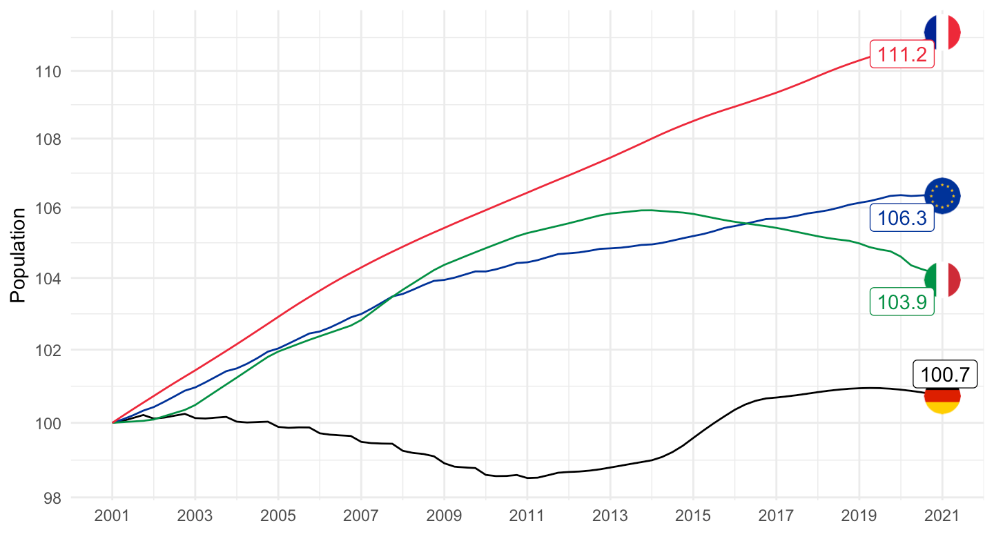

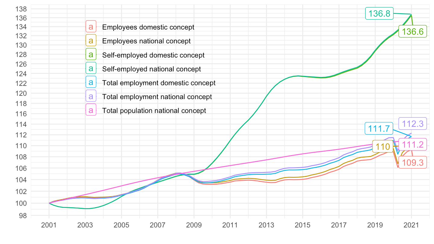
France Evolution

Max -

NSA

Code

namq_10_pe |>
  filter(geo == "FR",
         unit == "THS_PER",
         s_adj == "NSA") |>
  
  quarter_to_date() |>
  group_by(na_item) |>
  mutate(values = 100*values/values[1]) %>%
  select_if(~ n_distinct(.) > 1) |>
  ggplot() + ylab("Indice des prix, Ensemble") + xlab("") + theme_minimal() +
  geom_line(aes(x = date, y = values, color = Na_item)) +
  theme_minimal() +
  scale_x_date(breaks = seq(1909, 2100, 5) |> paste0("-01-01") |> as.Date(),
               labels = date_format("%Y")) +
  theme(legend.position = c(0.3, 0.7),
        legend.title = element_blank()) +
  scale_y_log10(breaks = seq(10, 300, 2),
                     labels = dollar_format(accuracy = 1, prefix = "")) +
  geom_label_repel(data = . %>% group_by(Na_item) %>% filter(date == max(date)), aes(x = date, y = values, label = round(values, 1), color = Na_item), show.legend = F)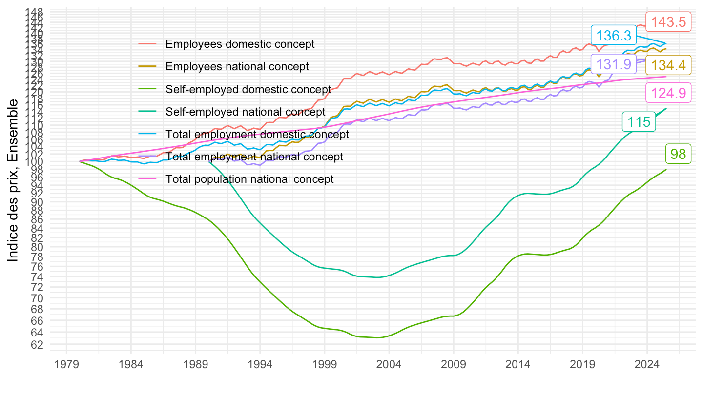

SA

Code

namq_10_pe |>
  filter(geo == "FR",
         unit == "THS_PER",
         s_adj == "SA") |>
  
  quarter_to_date() |>
  #filter(date >= as.Date("1999-01-01")) %>%
  group_by(na_item) |>
  mutate(values = 100*values/values[1]) %>%
  select_if(~ n_distinct(.) > 1) |>
  ggplot() + ylab("") + xlab("") + theme_minimal() +
  geom_line(aes(x = date, y = values, color = Na_item)) +
  theme_minimal() +
  scale_x_date(breaks = seq(1979, 2100, 5) |> paste0("-01-01") |> as.Date(),
               labels = date_format("%Y")) +
  theme(legend.position = c(0.3, 0.7),
        legend.title = element_blank()) +
  scale_y_log10(breaks = seq(10, 300, 2),
                     labels = dollar_format(accuracy = 1, prefix = "")) +
  geom_label_repel(data = . %>% group_by(Na_item) %>% filter(date == max(date)), aes(x = date, y = values, label = round(values, 1), color = Na_item))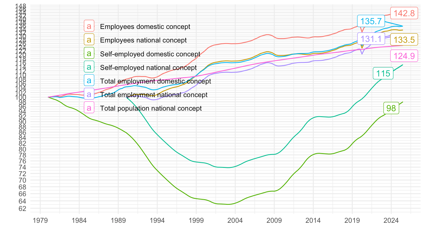

1999 -

NSA

Code

namq_10_pe |>
  filter(geo == "FR",
         unit == "THS_PER",
         s_adj == "NSA") |>
  
  quarter_to_date() |>
  filter(date >= as.Date("1999-01-01")) |>
  group_by(na_item) |>
  mutate(values = 100*values/values[1]) %>%
  select_if(~ n_distinct(.) > 1) |>
  ggplot() + ylab("Indice des prix, Ensemble") + xlab("") + theme_minimal() +
  geom_line(aes(x = date, y = values, color = Na_item)) +
  theme_minimal() +
  scale_x_date(breaks = seq(1999, 2100, 5) |> paste0("-01-01") |> as.Date(),
               labels = date_format("%Y")) +
  theme(legend.position = c(0.3, 0.8),
        legend.title = element_blank()) +
  scale_y_log10(breaks = seq(10, 300, 2),
                     labels = dollar_format(accuracy = 1, prefix = "")) +
  geom_label_repel(data = . %>% group_by(Na_item) %>% filter(date == max(date)), aes(x = date, y = values, label = round(values, 1), color = Na_item))

SA

Code

namq_10_pe |>
  filter(geo == "FR",
         unit == "THS_PER",
         s_adj == "SA") |>
  
  quarter_to_date() |>
  filter(date >= as.Date("1999-01-01")) |>
  group_by(na_item) |>
  mutate(values = 100*values/values[1]) %>%
  select_if(~ n_distinct(.) > 1) |>
  ggplot() + ylab("") + xlab("") + theme_minimal() +
  geom_line(aes(x = date, y = values, color = Na_item)) +
  theme_minimal() +
  scale_x_date(breaks = seq(1999, 2100, 5) |> paste0("-01-01") |> as.Date(),
               labels = date_format("%Y")) +
  theme(legend.position = c(0.3, 0.7),
        legend.title = element_blank()) +
  scale_y_log10(breaks = seq(10, 300, 2),
                     labels = dollar_format(accuracy = 1, prefix = "")) +
  geom_label_repel(data = . %>% group_by(Na_item) %>% filter(date == max(date)), aes(x = date, y = values, label = round(values, 1), color = Na_item))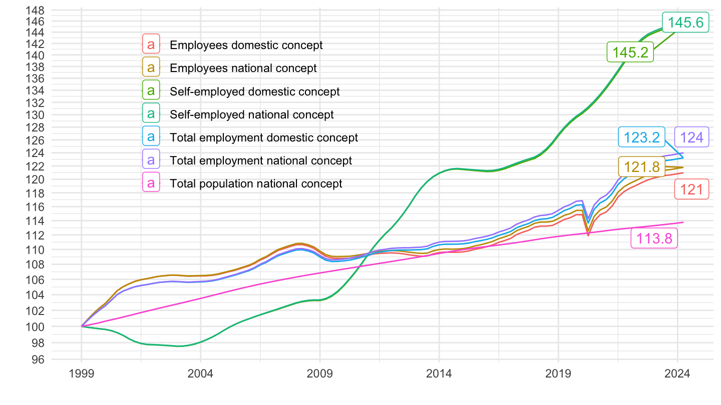

2001-2021

NSA

Code

namq_10_pe |>
  filter(geo == "FR",
         unit == "THS_PER",
         s_adj == "NSA") |>
  
  quarter_to_date() |>
  filter(date >= as.Date("2001-01-01"),
         date <= as.Date("2021-01-01")) |>
  group_by(na_item) |>
  mutate(values = 100*values/values[1]) %>%
  select_if(~ n_distinct(.) > 1) |>
  ggplot() + ylab("Indice des prix, Ensemble") + xlab("") + theme_minimal() +
  geom_line(aes(x = date, y = values, color = Na_item)) +
  theme_minimal() +
  scale_x_date(breaks = seq(1999, 2100, 5) |> paste0("-01-01") |> as.Date(),
               labels = date_format("%Y")) +
  theme(legend.position = c(0.3, 0.7),
        legend.title = element_blank()) +
  scale_y_log10(breaks = seq(10, 300, 2),
                     labels = dollar_format(accuracy = 1, prefix = "")) +
  geom_label_repel(data = . %>% group_by(Na_item) %>% filter(date == max(date)), aes(x = date, y = values, label = round(values, 1), color = Na_item), show.legend = F)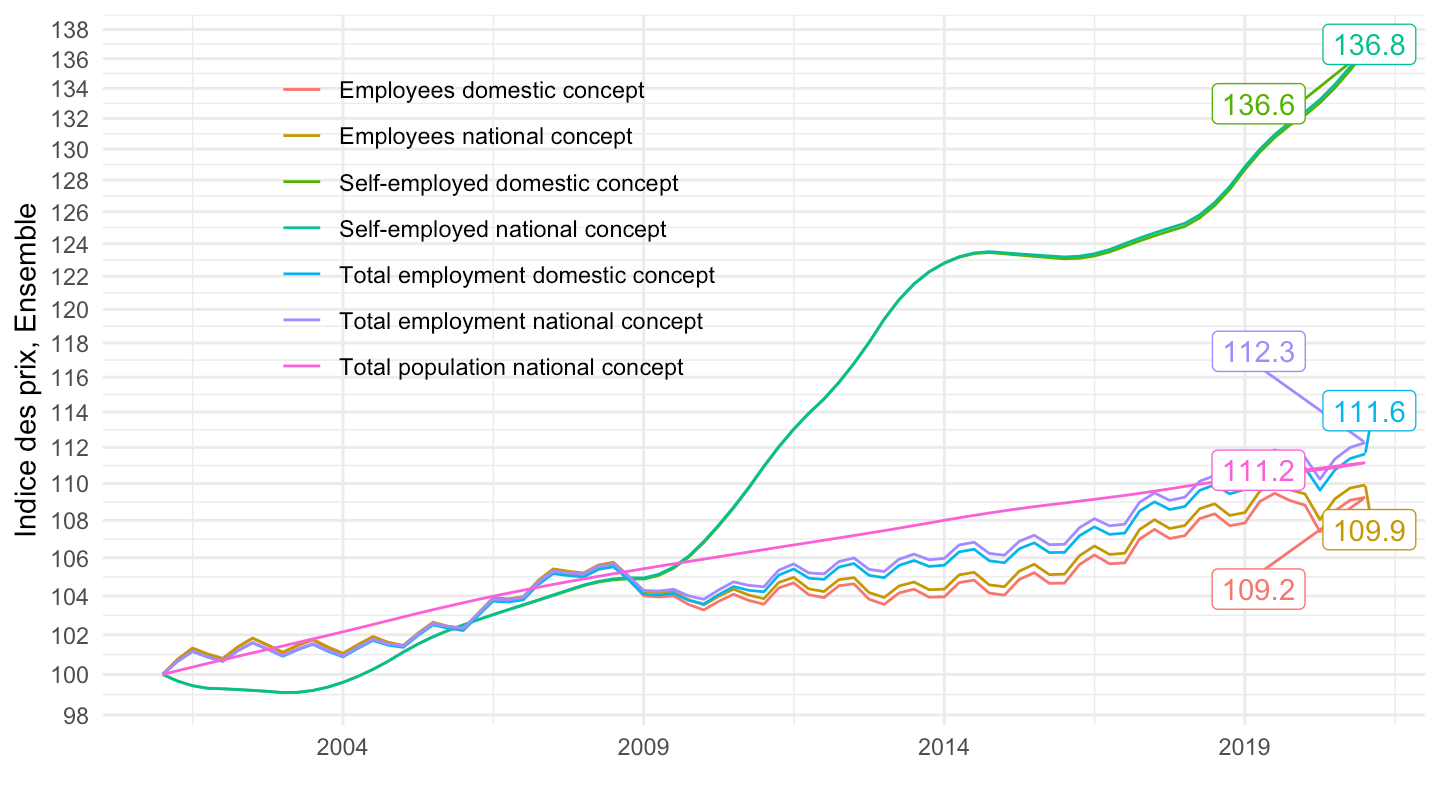

SA

Code

namq_10_pe |>
  filter(geo == "FR",
         unit == "THS_PER",
         s_adj == "SA") |>
  
  quarter_to_date() |>
  filter(date >= as.Date("2001-01-01"),
         date <= as.Date("2021-01-01")) |>
  group_by(na_item) |>
  mutate(values = 100*values/values[1]) %>%
  select_if(~ n_distinct(.) > 1) |>
  ggplot() + ylab("") + xlab("") + theme_minimal() +
  geom_line(aes(x = date, y = values, color = Na_item)) +
  theme_minimal() +
  scale_x_date(breaks = seq(2001, 2100, 2) |> paste0("-01-01") |> as.Date(),
               labels = date_format("%Y")) +
  theme(legend.position = c(0.3, 0.7),
        legend.title = element_blank()) +
  scale_y_log10(breaks = seq(10, 300, 2),
                     labels = dollar_format(accuracy = 1, prefix = "")) +
  geom_label_repel(data = . %>% group_by(Na_item) %>% filter(date == max(date)), aes(x = date, y = values, label = round(values, 1), color = Na_item))