Average full time adjusted salary per employee

Data - Eurostat

Author

François Geerolf

Info

Last observation: Annual: 2024 (N = 56)

First observation: Annual: 1995 (N = 26)

Last data update: 11 aoû 2026, 18:57. Last compile: 12 aoû 2026, 01:44

Structure

Population Table

English

Code

nama_10_fte |>
  filter(time %in% c(max(time), "2019", "2009", "1999", "1989"),
         unit == "EUR") |>
  select(geo, time, values) |>
  mutate(values = round(values/1000, 1)) |>
  
  spread(time, values) |>
  arrange(- `2019`) %>%
  {if (is_html_output()) datatable(., filter = 'top', rownames = F) else .}

French

Code

geo <- read_parquet("geo_fr.parquet")
nama_10_fte |>
  filter(time %in% c(max(time), "2019", "2009", "1999", "1989"),
         unit == "EUR") |>
  select(geo, time, values) |>
  mutate(values = round(values/1000, 1)) |>
  
  spread(time, values) |>
  arrange(- `2019`) %>%
  {if (is_html_output()) datatable(., filter = 'top', rownames = F) else .}

Countries

Poland, Germany, Hungary

Code

geo <- read_parquet("geo.parquet")
nama_10_fte |>
  filter(geo %in% c("PL", "DE", "HU"),
         unit == "EUR") |>
  select(geo, Geo, time, values) |>
  year_to_date() |>
  
  ggplot() + geom_line(aes(x = date, y = values/1000, color = Geo)) +
  theme_minimal()  +
  scale_x_date(breaks = as.Date(paste0(seq(1960, 2100, 5), "-01-01")),
               labels = date_format("%Y")) +
  theme(legend.position = c(0.35, 0.85),
        legend.title = element_blank()) +
  xlab("") + ylab("") +
  scale_y_continuous(breaks = seq(-30, 150, 10))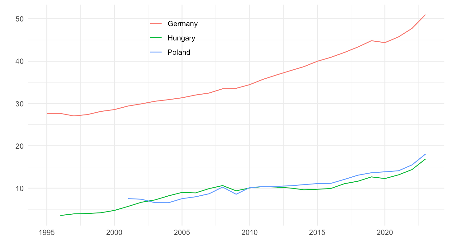

France, Italy, Spain

Code

nama_10_fte |>
  filter(geo %in% c("FR", "IT", "ES"),
         unit == "EUR") |>
  select(geo, Geo, time, values) |>
  year_to_date() |>

  ggplot() + geom_line(aes(x = date, y = values/1000, color = Geo)) +
  theme_minimal()  +
  scale_x_date(breaks = as.Date(paste0(seq(1960, 2100, 5), "-01-01")),
               labels = date_format("%Y")) +
  theme(legend.position = c(0.35, 0.85),
        legend.title = element_blank()) +
  xlab("") + ylab("") +
  scale_y_continuous(breaks = seq(-30, 150, 10))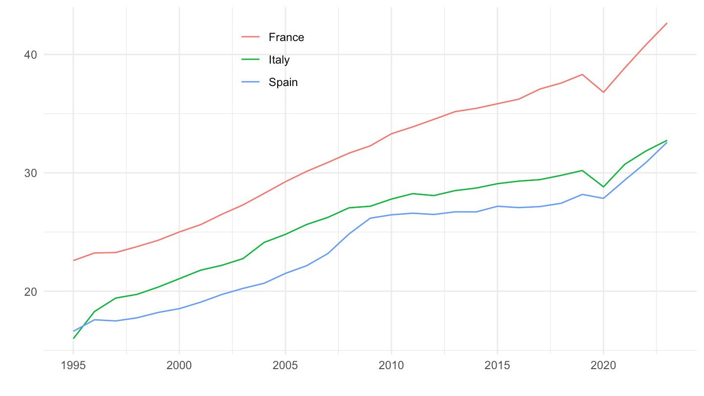

Sweden, Denmark, Finland

Code

nama_10_fte |>
  filter(geo %in% c("SE", "DK", "FI"),
         unit == "EUR") |>
  select(geo, Geo, time, values) |>
  year_to_date() |>
  mutate(values = values/1000) |>
  left_join(colors, by = c("Geo" = "country")) |>
  ggplot() + geom_line(aes(x = date, y = values, color = color)) +
  theme_minimal() + scale_color_identity() + add_flags +
  scale_x_date(breaks = as.Date(paste0(seq(1960, 2100, 5), "-01-01")),
               labels = date_format("%Y")) +
  xlab("") + ylab("Average full-time adjusted salary (Th. €)")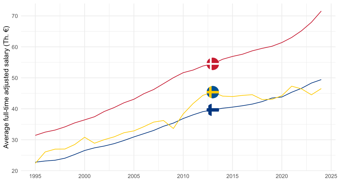

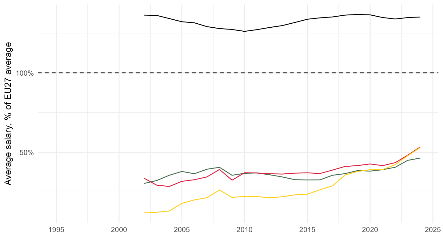
Wage Convergence

Poland, Romania, Hungary vs. Germany (% of EU27 Average)

Code

nama_10_fte |>
  filter(geo %in% c("PL", "RO", "HU", "DE", "EU27_2020"),
         unit == "EUR") |>
  select(geo, time, values) |>
  spread(geo, values) |>
  mutate(PL = PL/EU27_2020, RO = RO/EU27_2020, HU = HU/EU27_2020, DE = DE/EU27_2020) |>
  select(time, PL, RO, HU, DE) |>
  gather(geo, values, -time) |>
  left_join(distinct(nama_10_fte, geo, Geo), by = "geo") |>
  year_to_date() |>
  left_join(colors, by = c("Geo" = "country")) |>
  ggplot() + geom_line(aes(x = date, y = values, color = color)) +
  theme_minimal() + scale_color_identity() + add_flags +
  scale_x_date(breaks = as.Date(paste0(seq(1995, 2100, 5), "-01-01")),
               labels = date_format("%Y")) +
  xlab("") + ylab("Average salary, % of EU27 average") +
  scale_y_continuous(labels = scales::percent_format(accuracy = 1)) +
  geom_hline(yintercept = 1, linetype = "dashed", color = "black")