Analyzing inflation by household categories: some methodological issues
inflation
purchasing power
methodology
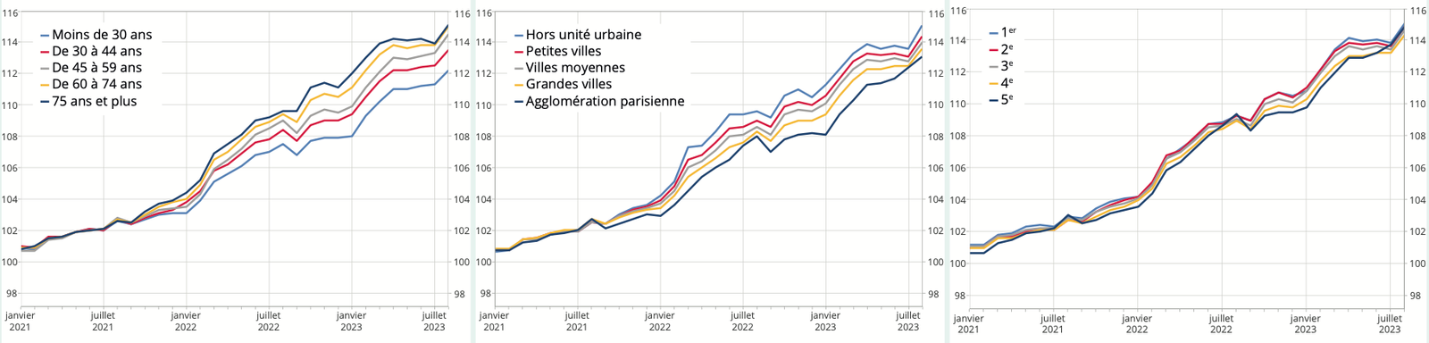
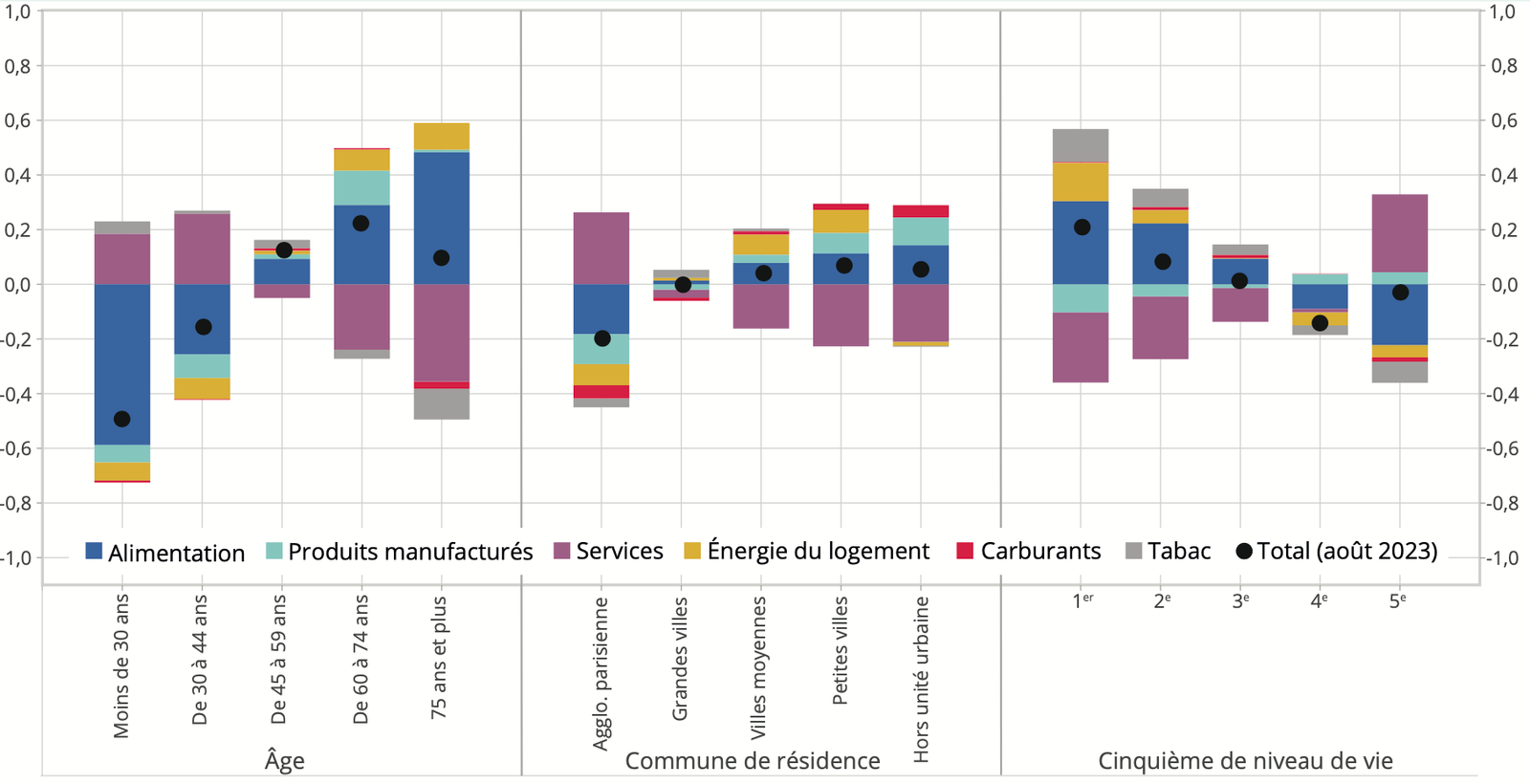
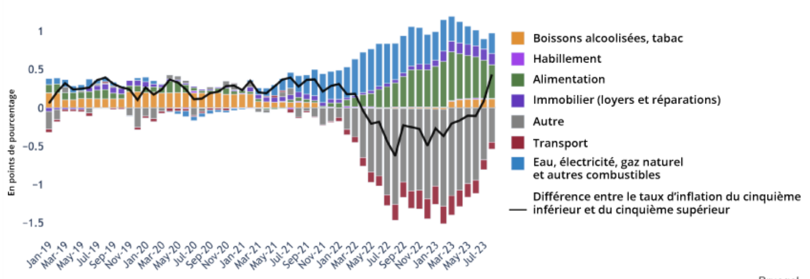
According to Insee’s Economic Outlook from October 2023, household inflation levels depend very little on income: the richest households experience roughly the same level of inflation as the poorest households. By contrast, inflation is significantly higher for older individuals and for those living in rural areas compared to Paris (Figure 1). Other studies by Bruegel, Insee, the Trésor, the OFCE, the IMF, and the Conseil d’Analyse Économique1 appear to confirm this finding: according to Bruegel, the poorest households have even faced lower inflation than the richest until very recently (Figure 3). Work by Insee, Bruegel, and the OFCE has also proposed a sectoral decomposition of the inflation gap: while food and energy behave as expected—generating higher inflation for poorer households—this effect is almost entirely offset by the consumption of services according to Insee (Figure 2), an “other” category in Bruegel (Figure 3), and a “remainder” category in the OFCE (Figure 4).
A questionable decomposition
The aforementioned studies decompose the gap between the average inflation of a household category \(m\) (\(\pi^m\)) and the average inflation for all households (\(\pi\)) as a function of the differences between the budget share of goods \(b\) consumed by this household category \(m\) (\(\omega_b^m\)) and the budget share of goods \(b\) consumed by all households (\(\omega_b\)), according to the following formula:
\[ \pi^m - \pi = \sum_b (\omega_b^m - \omega_b)\cdot \pi_b \tag{1}\]
where \(\pi_b\) is the average inflation for the category of goods \(b\).
This decomposition is questionable because it assumes that a good with zero inflation (\(\pi_b=0\)) has a zero contribution to the inflation differential. Yet in a context of high average inflation, a good with zero inflation contributes to lowering inflation, and even more so for households that consume this good in larger quantities. The decomposition should therefore intuitively highlight the differential between the inflation on this good \(\pi_b\) and average inflation \(\pi\): a good with lower-than-average inflation and consumed more heavily by a household contributes to reducing that household’s inflation relative to the average. This is especially true if the inflation on this good is zero while the average inflation is high.
We therefore propose an alternative decomposition that introduces the gap to average inflation: \[ \pi^m - \pi = \sum_b (\omega_b^m - \omega_b)\cdot (\pi_b-\pi). \tag{2}\]
This new decomposition ultimately shows that if the inflation of good \(b\) is higher (lower) than average inflation, and its budget share is greater for a household relative to the average, its contribution to the inflation gap will be positive (negative) and smaller than in the first measure2. The difference between Equation 1 and Equation 2 will be all the greater the higher the inflation. Thus, Equation 1 overestimates contributions to inflation. With Equation 2, we recover another very intuitive result: if the inflation on a good \(b\) equals average inflation, then this good cannot contribute to the inflation differential3.
Thus, in August 2023, with this new method, fuels—whose inflation was lower than average inflation (2.3% versus 4.9% respectively)—contributed to lowering inflation for residents of rural municipalities and for poor households, since they consume more fuel. By contrast, with Insee’s first method (Figure 2), fuels appeared to raise inflation for rural residents and poor households. Another example: still in August 2023, inflation was 9.9% for housing energy, about 5 points higher than overall inflation. All contributions of housing energy must therefore be divided by 2 with this new method. Overall, all the calculations made previously are thus modified.
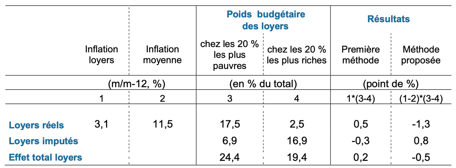
The main correction concerns rents actually paid by tenants (“real” rents). Inflation on rents is positive but currently much lower than overall inflation (partly thanks to rent cap policies): +3.1% over 2 years in November 2023, compared to +11.5% overall inflation according to the HICP4. According to Eurostat, the poorest 20% spend 17.5% of their budget on rent, compared to 2.5% for the richest 20%. According to the method of the previous studies, rents would appear to increase inflation for the poorest relative to the richest by about 0.5 points over 2 years. This is what Figure 3 shows, with a positive contribution of rents to the inflation gap. According to the proposed method, rents instead lower inflation for the poorest relative to the richest by about 1.3 points. This explains why, despite the regressive character of energy and food inflation, inflation appears very similar between the richest and the poorest.
The Exclusion of Owner-Occupied Housing Consumption
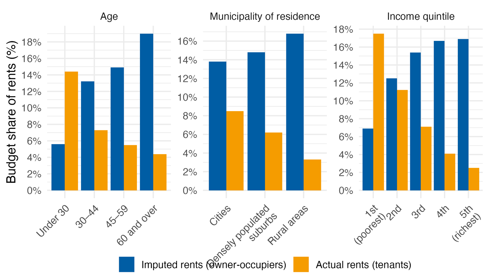
But is it true that the budget share of housing consumption among the poorest is 15% higher than that of the richest? No—if we also include the housing consumption of owner-occupiers, which takes the form of so-called “imputed” rents. According to Eurostat, “imputed” rents account for 6.9% of the budget for the bottom quintile, and 16.9% for the top quintile, due to a higher share of homeowners among richer households, as shown in Figure 5. Taking imputed rents for homeowners into account increases the inflation gap between the poorest and the richest by 0.8 points, via a reduction in the inflation of richer households that would otherwise be overstated. In the end, rents reduce the inflation of the poorest compared to the richest by only 0.5 points, rather than 1.3 points (Table 1). This is enough to make the inflation of the poorest higher than that of the richest, reversing the results of Figure 1.
What about other household categories? Compared with the figures from Figure 5, the gap between the inflation of those under 30 and those over 60 must itself be increased by about 1.1 percentage points over two years—a very significant correction. Here again, it is the inflation of older households that is otherwise overstated. Finally, the correction is less important for the gap between cities and rural areas, which must be increased by about 0.3 percentage points over two years—again via a downward adjustment of the inflation experienced in rural areas during this inflationary episode.
The “imputed” rents of owner-occupiers are in fact taken into account neither in the official measure of inflation (CPI, HICP), nor in the household-level inflation analyses presented above. Yet the question of whether the housing consumption of owner-occupiers should be included in the price index has long been a matter of debate (see the report of the CAE in 2008). An Insee blog from February 2020 defended its choice not to include owner-occupied housing in the CPI. As discussed in a note in February 2022, many of the arguments put forward in this blog were inaccurate: the “imputed” rents of owners are indeed part of consumption in national accounts, as well as from the point of view of economic theory. Moreover, owners bear many expenses linked to the occupation of their housing, which are not borne by tenants and do not increase the value of their real estate assets: routine housing maintenance expenditures to keep it in good condition, condominium charges, etc. The capital tied up in housing does not yield interest, which constitutes a loss of income and therefore a form of consumption equal to the amount that the owner could receive if they chose to rent out the dwelling. In fact, Insee’s position on this matter seems to have evolved recently, if one believes a recent interview with the Director General of Insee in the magazine Sociétal: “On the other hand, the use of real estate does fall under consumption. And in the consumer price index, rents are included—today, only those of actual tenants. One could add the rents of owner-occupiers.” The so-called “imputed” rents of owner-occupiers are moreover included in the CPI of the vast majority of countries5.
Bias due to inflation via the rise in commodity prices
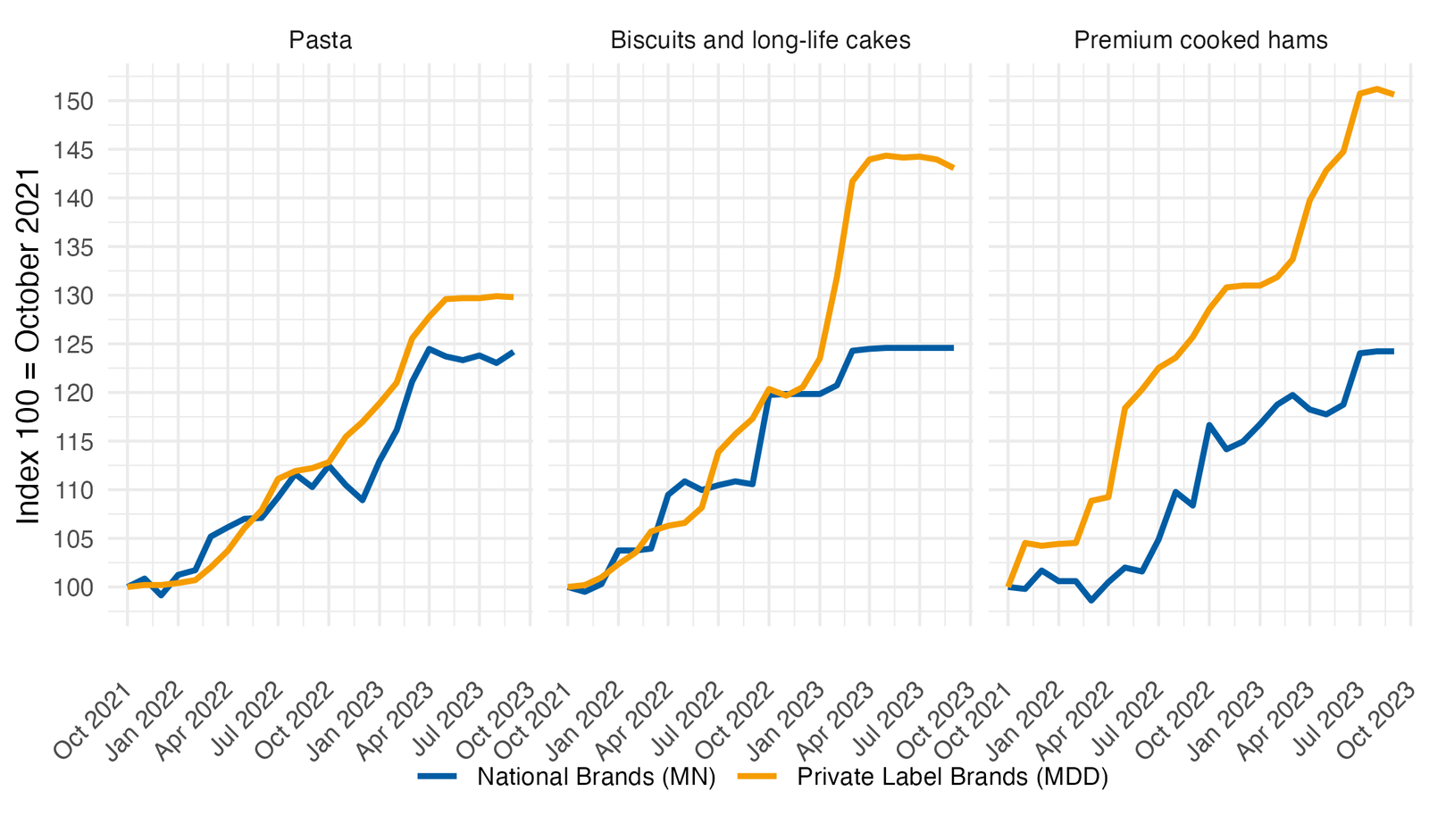
There is a final bias in the calculation of inflation by household categories, linked to the specific nature of inflation initially driven by commodities. Inflation through commodities affects households differently, even within a single category of goods available in the surveys (aggregation bias). Lower-quality goods with lower value added experience larger price increases following a commodity price shock. In food, producer prices for private-label (marques de distributeur) food products rise more rapidly (by 30 to 45%) than those of national brands (between 20 and 25%), as shown in Figure 6.
This is not surprising from a theoretical point of view, and the microeconomic data more generally confirm this6. Finally, inflation as measured here does not take into account substitution possibilities. These are greater for wealthier households, who can limit their inflation by substituting (buying less fish, trading down in quality). Such possibilities are more limited when the budget is already constrained.
In conclusion, analyzing inflation by household categories presents numerous methodological challenges that must be kept in mind before drawing economic policy conclusions. The official measurement of inflation does not account for housing consumption by owner-occupiers and therefore currently overestimates inflation for owner-occupiers in general: that of older households by about 1 percentage point over 2 years (both in absolute terms and relative to younger households), that of households living in rural areas by about 0.3 percentage points, and finally that of wealthier households by about 1 percentage point. Once this is taken into account, poorer households do in fact experience higher inflation than richer households, which aligns with intuition and qualitatively corresponds to the result obtained when considering only the effect of food and energy inflation. This is all the more true when food inflation is analyzed more finely, as it is greater for the less well-off than for the wealthier.
Footnotes
Claeys, G., L. Guetta-Jeanrenaud, C. McCaffrey, L. Welslau (2022) “Inflation inequality in the European Union and its drivers” Bruegel datasets, first published 26 October 2022 ; Insee (2022) Note de conjoncture, juin 2022 ; Bénassy-Quéré A. (2022). « Injuste inflation », Billet de la DG Trésor, septembre 2022 ; Madec P., Plane M., Sampognaro R. (2023) « Une analyse des mesures budgétaires et du pouvoir d’achat en France en 2022 et 2023 », OFCE Policy Brief n°112, février 2023 ; IMF (2022) “How Europe Can Protect the Poor from Surging Energy Prices” IMF Blog ; Jaravel X., I. Méjean, X. Ragot (2023) « Les politiques publiques face au retour de l’inflation » Note du CAE n°78 ; Astier J., X. Jaravel, M. Péron (2023) « Mesurer les effets hétérogènes de l’inflation sur les ménages » Focus du CAE n°99, juillet 2023. In contrast, see Allègre G., Geerolf F., Timbeau X. (2022) « Inflation en Europe : les conséquences sociales de la guerre en Ukraine » Blog de l’OFCE, July 2022.↩︎
If the budget share of a good \(b\) is lower in a household’s expenditures than in the average household, then its contribution will be negative (positive) and smaller if the inflation of good \(b\) is higher (lower) than average inflation.↩︎
Note that the sum of the terms of this decomposition is the same since the sum of the weights equals 1:
\[\sum_b (\omega_b^m - \omega_b)\cdot (-\pi)=\left(\sum_b \omega_b^m - \sum_b \omega_b\right)\cdot (-\pi)=0.\] There is in fact an infinity of decompositions with the contribution of good \(b\) to inflation equal to \((\omega_b^m - \omega_b)\cdot (\pi_b-c)\). The decomposition used by the aforementioned studies amounts to choosing \(c=0\), while we propose instead to take \(c=\pi\).↩︎+10.5% according to Insee’s CPI, which takes reimbursed health expenditures into account—this lowers measured inflation compared to the HICP but seems debatable, see here, p. 2.↩︎
Some references in this debate : Ourliac B. (2020). « Mais si, l’Insee prend bien en compte le logement dans l’inflation ! » Blog de l’Insee, 4 février 2020. Geerolf F. (2022). « Quelques remarques au sujet du Blog de l’Insee du 4 février 2020 : « Mais si, l’Insee prend bien en compte le logement dans l’inflation ! ». Document de travail, 22 février 2022. Tavernier J-L. (2022). Interview. De l’excès de demande mondiale de biens à un monde en tension sur l’offre. Le retour de l’inflation. Sociétal, 4ème trimestre 2022, 44-51.↩︎
For example: Sangani, K (2023), “Pass-through in levels and the unequal incidence of commodity shocks”, Working Paper.↩︎