Fixed assets by activity and by asset, ISIC rev4

Data - OECD

Author

Info

source	dataset	Title	.html	.rData
oecd	SNA_TABLE9A	Fixed assets by activity and by asset, ISIC rev4	2026-01-11	2023-12-20

LAST_DOWNLOAD

Code

tibble(LAST_DOWNLOAD = as.Date(file.info("~/iCloud/website/data/oecd/SNA_TABLE9A.RData")$mtime)) %>%
  print_table_conditional()

LAST_DOWNLOAD
2023-12-20

LAST_COMPILE

LAST_COMPILE
2026-01-15

Last

TRANSACT

Code

SNA_TABLE9A %>%
  left_join(SNA_TABLE9A_var$TRANSACT, by = "TRANSACT") %>%
  group_by(TRANSACT, Transact) %>%
  summarise(Nobs = n()) %>%
  arrange(-Nobs) %>%
  print_table_conditional()

LOCATION

Code

SNA_TABLE9A %>%
  left_join(SNA_TABLE9A_var$LOCATION, by = "LOCATION") %>%
  group_by(LOCATION, Location) %>%
  summarise(Nobs = n()) %>%
  arrange(-Nobs) %>%
  mutate(Flag = gsub(" ", "-", str_to_lower(gsub(" ", "-", Location))),
         Flag = paste0('<img src="../../icon/flag/vsmall/', Flag, '.png" alt="Flag">')) %>%
  select(Flag, everything()) %>%
  {if (is_html_output()) datatable(., filter = 'top', rownames = F, escape = F) else .}

ACTIVITY

Code

SNA_TABLE9A %>%
  left_join(SNA_TABLE9A_var$ACTIVITY, by = "ACTIVITY") %>%
  group_by(ACTIVITY, Activity) %>%
  summarise(Nobs = n()) %>%
  arrange(-Nobs) %>%
  print_table_conditional()

MEASURE

Code

SNA_TABLE9A %>%
  left_join(SNA_TABLE9A_var$MEASURE, by = "MEASURE") %>%
  group_by(MEASURE, Measure) %>%
  summarise(Nobs = n()) %>%
  arrange(-Nobs) %>%
  print_table_conditional()

MEASURE	Measure	Nobs
C	Current prices	996828
VP	Constant prices, previous year prices	901237
V	Constant prices, national base year	787733
DOB	Deflator	757575

Equipment, Fixed Assets

United States

Code

SNA_TABLE9A %>%
  rename(obsTime = Time, obsValue = ObsValue) %>%
  mutate(obsValue = as.numeric(obsValue)) %>%
  filter(TRANSACT %in% c("N1113NA", "N1113ONA", "N11131NA", "B1_GE"),
         ACTIVITY == "VTOT",
         MEASURE == "C",
         LOCATION == "USA") %>%
  left_join(SNA_TABLE9A_var$TRANSACT, by = "TRANSACT") %>%
  year_to_date %>%
  select(date, Transact, obsValue) %>%
  spread(Transact, obsValue) %>%
  rename(GDP = `Gross domestic product (expenditure approach)`) %>%
  mutate_at(vars(-GDP, -date), funs(./ GDP)) %>%
  select(-GDP) %>%
  gather(Transact, value, -date) %>%
  ggplot(.) + geom_line(aes(x = date, y = value, color = Transact)) +
  theme_minimal() +
  theme(legend.position = c(0.7, 0.3),
        legend.title = element_blank(),
        legend.text = element_text(size = 8),
        legend.key.size = unit(0.9, 'lines')) +
  scale_y_continuous(breaks = 0.01*seq(0, 500, 10),
                     labels = scales::percent_format(accuracy = 1),
                     limits = c(0, 0.6)) +
  scale_x_date(breaks = seq(1700, 2020, 5) %>% paste0(., "-01-01") %>% as.Date,
               limits =  c(1970, 2010) %>% paste0(., "-01-01") %>% as.Date,
               labels = date_format("%Y")) + 
  xlab("") + ylab("% of GDP")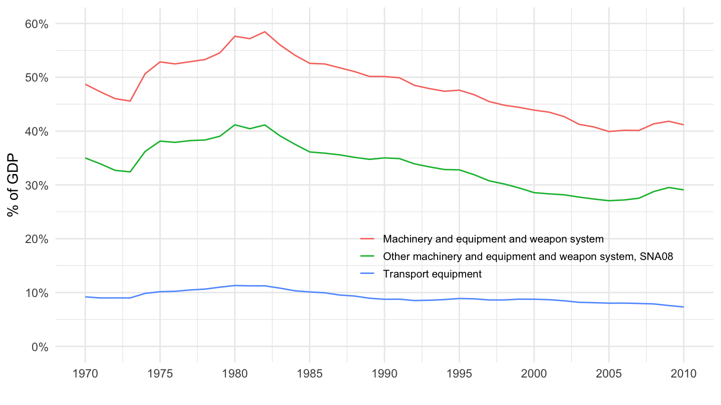

Net Fixed Assets

png

Code

include_graphics3("bib/oecd/SNA_TABLE9A_ex1.png")

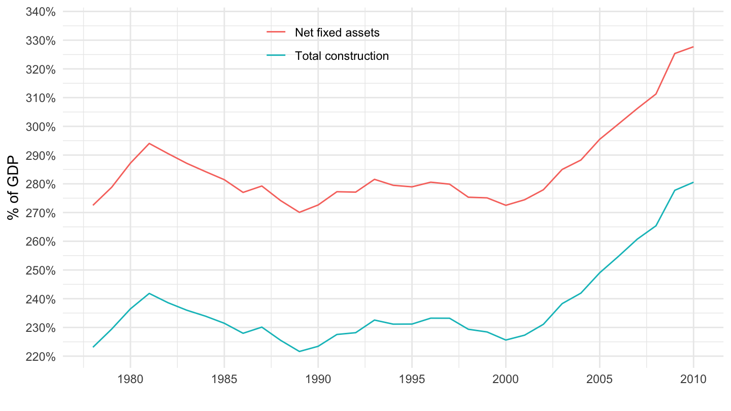
U.S. Net fixed Assets, Construction

Code

SNA_TABLE9A %>%
  rename(obsTime = Time, obsValue = ObsValue) %>%
  mutate(obsValue = as.numeric(obsValue)) %>%
  filter(TRANSACT %in% c("N111XNA", "N11NA", "B1_GE"),
         ACTIVITY == "VTOT",
         MEASURE == "C",
         LOCATION == "USA") %>%
  left_join(SNA_TABLE9A_var$TRANSACT, by = "TRANSACT") %>%
  year_to_date %>%
  select(date, Transact, obsValue) %>%
  spread(Transact, obsValue) %>%
  rename(GDP = `Gross domestic product (expenditure approach)`) %>%
  mutate_at(vars(-GDP, -date), funs(./ GDP)) %>%
  select(-GDP) %>%
  gather(Transact, value, -date) %>%
  ggplot(.) + geom_line(aes(x = date, y = value, color = Transact)) +
  theme_minimal() +
  theme(legend.position = c(0.4, 0.9),
        legend.title = element_blank()) +
  scale_y_continuous(breaks = 0.01*seq(0, 500, 10),
                     labels = scales::percent_format(accuracy = 1)) +
  scale_x_date(breaks = seq(1700, 2020, 5) %>% paste0(., "-01-01") %>% as.Date,
               limits =  c(1978, 2018) %>% paste0(., "-01-01") %>% as.Date,
               labels = date_format("%Y")) + 
  xlab("") + ylab("% of GDP")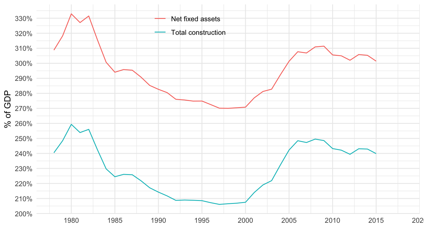

France Net fixed Assets, Construction

Code

SNA_TABLE9A %>%
  rename(obsTime = Time, obsValue = ObsValue) %>%
  mutate(obsValue = as.numeric(obsValue)) %>%
  filter(TRANSACT %in% c("N111XNA", "N11NA", "B1_GE"),
         ACTIVITY == "VTOT",
         MEASURE == "C",
         LOCATION == "FRA") %>%
  left_join(SNA_TABLE9A_var$TRANSACT, by = "TRANSACT") %>%
  year_to_date %>%
  select(date, Transact, obsValue) %>%
  spread(Transact, obsValue) %>%
  rename(GDP = `Gross domestic product (expenditure approach)`) %>%
  mutate_at(vars(-GDP, -date), funs(./ GDP)) %>%
  select(-GDP) %>%
  gather(Transact, value, -date) %>%
  ggplot(.) + geom_line(aes(x = date, y = value, color = Transact)) +
  theme_minimal() +
  theme(legend.position = c(0.4, 0.9),
        legend.title = element_blank()) +
  scale_y_continuous(breaks = 0.01*seq(0, 500, 10),
                     labels = scales::percent_format(accuracy = 1)) +
  scale_x_date(breaks = seq(1700, 2020, 5) %>% paste0(., "-01-01") %>% as.Date,
               limits =  c(1978, 2010) %>% paste0(., "-01-01") %>% as.Date,
               labels = date_format("%Y")) + 
  xlab("") + ylab("% of GDP")