| source | dataset | Title | .html | .rData |
|---|---|---|---|---|
| oecd | SNA_TABLE8A | Capital formation by activity ISIC rev4 | 2026-07-24 | 2024-06-30 |
Capital formation by activity ISIC rev4
Data - OECD
Info
LAST_DOWNLOAD
Code
tibble(LAST_DOWNLOAD = as.Date(file.info("~/iCloud/website/data/oecd/SNA_TABLE8A.RData")$mtime)) %>%
print_table_conditional()| LAST_DOWNLOAD |
|---|
| 2024-06-30 |
LAST_COMPILE
| LAST_COMPILE |
|---|
| 2026-07-26 |
Last
| obsTime | Nobs |
|---|---|
| 2023 | 3 |
Layout
- OECD Website. html
Germany

France
Transaction, Activity
TRANSACT
Code
SNA_TABLE8A %>%
  left_join(SNA_TABLE8A_var$TRANSACT, by = "TRANSACT") %>%
  group_by(TRANSACT, Transact) %>%
  summarise(Nobs = n()) %>%
  arrange(-Nobs) %>%
print_table_conditional| TRANSACT | Transact | Nobs |
|---|---|---|
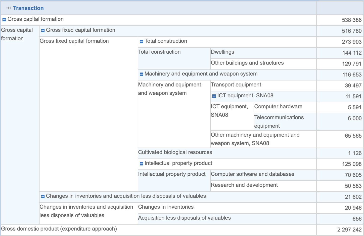
| P51A | Gross fixed capital formation | 310270 |
| P51N1112A | Other buildings and structures | 236119 |
| P51N1113A | Machinery and equipment and weapon system | 235824 |
| P51N11131A | Transport equipment | 235276 |
| P51N112A | Intellectual property product | 233380 |
| P51N111XA | Total construction | 225436 |
| P51N1113OA | Other machinery and equipment and weapon system, SNA08 | 214667 |
| P51N1113IA | ICT equipment, SNA08 | 201134 |
| P51N1122A | Computer software and databases | 187599 |
| P51N1124A | Research and development | 179873 |
| P51N111321A | Computer hardware | 169169 |
| P51N111322A | Telecommunications equipment | 166764 |
| P51N1111A | Dwellings | 163576 |
| P51N1114A | Cultivated biological resources | 150468 |
| P5A | Gross capital formation | 84241 |
| P52A | Changes in inventories | 66915 |
| P52_P53A | Changes in inventories and acquisition less disposals of valuables | 42339 |
| P53A | Acquisition less disposals of valuables | 22914 |
| P51N11221A | Computer software | 16693 |
| P51N1123A | Entertainment, literary and artistic originals | 7461 |
| P51N1121A | Mineral exploration and evaluation | 4036 |
| B1_GE | Gross domestic product (expenditure approach) | 2619 |
| P51N1129A | Other intellectual property products | 1149 |
| P51N11222A | NA | 750 |
| P51N11132A | Other machinery and equipment, SNA93 | 43 |
ACTIVITY
Code
SNA_TABLE8A %>%
  left_join(SNA_TABLE8A_var$ACTIVITY, by = "ACTIVITY") %>%
  group_by(ACTIVITY, Activity) %>%
  summarise(Nobs = n()) %>%
  arrange(-Nobs) %>%
  print_table_conditional
MEASURE
Code
SNA_TABLE8A %>%
  left_join(SNA_TABLE8A_var$MEASURE, by = "MEASURE") %>%
  group_by(MEASURE, Measure) %>%
  summarise(Nobs = n()) %>%
  arrange(-Nobs) %>%
print_table_conditional| MEASURE | Measure | Nobs |
|---|---|---|
| C | Current prices | 899431 |
| VP | Constant prices, previous year prices | 820993 |
| V | Constant prices, national base year | 757030 |
| DOB | Deflator | 622434 |
| VOB | Constant prices, OECD base year | 58827 |
LOCATION
Code
SNA_TABLE8A %>%
  left_join(SNA_TABLE8A_var$LOCATION, by = "LOCATION") %>%
  group_by(LOCATION, Location) %>%
  summarise(Nobs = n()) %>%
  arrange(-Nobs) %>%
  mutate(Flag = gsub(" ", "-", str_to_lower(gsub(" ", "-", Location))),
         Flag = paste0('<img src="../../icon/flag/vsmall/', Flag, '.png" alt="Flag">')) %>%
  select(Flag, everything()) %>%
  {if (is_html_output()) datatable(., filter = 'top', rownames = F, escape = F) else .}
obsTime
Code
SNA_TABLE8A %>%
  group_by(obsTime) %>%
  summarise(Nobs = n()) %>%
  arrange(desc(obsTime)) %>%
  print_table_conditional
Components
Inventories
Investment Rate by Sector
France, Germany, USA
Code
SNA_TABLE8A %>%
  filter(MEASURE == "C",
         LOCATION %in% c("USA", "FRA", "DEU"),
         TRANSACT %in% c("P51A", "B1_GE"),
         obsTime == "2016") %>%
  left_join(SNA_TABLE8A_var$ACTIVITY, by = "ACTIVITY") %>%
  select(LOCATION, TRANSACT, ACTIVITY, Activity, obsValue) %>%
  arrange(TRANSACT) %>%
  mutate(obsValue = obsValue/obsValue[TRANSACT == "B1_GE"]) %>%
  filter(TRANSACT != "B1_GE") %>%
  spread(LOCATION, obsValue) %>%
  select(-1) %>%
  mutate_at(vars(3:5), funs(ifelse(!is.na(.), paste0(round(100*., digits = 1), "%"), ""))) %>%
  print_table_conditional
GFCF, All Types
All Types; France, United States, Germany
Code
SNA_TABLE8A %>%
  filter(ACTIVITY == "VTOT",
         MEASURE == "C",
         LOCATION %in% c("USA", "FRA", "DEU")) %>%
  left_join(SNA_TABLE8A_var$TRANSACT, by = "TRANSACT") %>%
  left_join(SNA_TABLE8A_var$LOCATION, by = "LOCATION") %>%
  rename(`Type of Fixed Asset` = Transact) %>%
  filter(obsTime == 2016) %>%
  select(TRANSACT, `Type of Fixed Asset`, Location, obsValue) %>%
  arrange(TRANSACT) %>%
  mutate(Location = gsub(" ", "-", str_to_lower(gsub(" ", "-", Location))),
         Location = paste0('<img src="../../icon/flag/vsmall/', Location, '.png" alt="Flag">')) %>%
  group_by(Location) %>%
  spread(Location, obsValue) %>%
  mutate_at(vars(3:5), funs(ifelse(!is.na(.), paste0(round(100*. / .[1], digits = 1), "%"), ""))) %>%
  {if (is_html_output()) datatable(., filter = 'top', rownames = F, escape = F) else .}
All Countries; GFCF, IPP, Machinery, Other Buildings
Code
SNA_TABLE8A %>%
  filter(TRANSACT %in% c("B1_GE", "P51N1113A", "P51A",
                         "P51N112A", "P51N1111A", "P51N1112A"),
         ACTIVITY == "VTOT",
         MEASURE == "C") %>%
  left_join(SNA_TABLE8A_var$LOCATION, by = "LOCATION") %>%
  left_join(SNA_TABLE8A_var$TRANSACT, by = "TRANSACT") %>%
  mutate(Transact = case_when(Transact == "Gross fixed capital formation" ~ "GFCF",
                                    Transact == "Intellectual property product" ~ "IPP",
                                    Transact == "Machinery and equipment and weapon system" ~ "Machinery, Equip",
                                    Transact == "Other buildings and structures" ~ "Other Buildings",
                                    T ~ Transact)) %>%
  filter(obsTime == 2016) %>%
  select(Location, Transact, obsValue) %>%
  spread(Transact, obsValue) %>%
  filter(!is.na(`IPP`)) %>%
  rename(GDP = `Gross domestic product (expenditure approach)`) %>%
  mutate_at(vars(-GDP, -Location), funs(paste0(round(100*./ GDP, digits = 1), "%"))) %>%
  mutate_all(funs(gsub("NA%", "", .))) %>%
  select(-GDP) %>%
  select(Location, GFCF, everything()) %>%
  arrange(Location) %>%
  filter(`GFCF` != "") %>%
  mutate(Flag = gsub(" ", "-", str_to_lower(gsub(" ", "-", Location))),
         Flag = paste0('<img src="../../icon/flag/vsmall/', Flag, '.png" alt="Flag">')) %>%
  select(Flag, everything()) %>%
  {if (is_html_output()) datatable(., filter = 'top', rownames = F, escape = F) else .}
Individual Countries
Germany
Main Components
Code
SNA_TABLE8A %>%
  filter(ACTIVITY == "VTOT",
         MEASURE == "C",
         TRANSACT %in% c("P51N1111A", "P51N1112A", "P51N1113A", "P51N112A"),
         LOCATION == "DEU") %>%
  left_join(SNA_TABLE8A_var$TRANSACT, by = "TRANSACT") %>%
  left_join(B1_GE_C, by = c("LOCATION", "obsTime")) %>%
  year_to_date %>%
  ggplot + theme_minimal() + ylab("% of GDP") + xlab("") +
  geom_line(aes(x = date, y = obsValue / B1_GE_C, color = Transact)) +
  scale_y_continuous(breaks = 0.01*seq(0, 1300, 1),
                     labels = scales::percent_format(accuracy = 1),
                     limits = c(0.02, 0.1)) +
  scale_x_date(breaks = seq(1920, 2100, 2) %>% paste0("-01-01") %>% as.Date,
               labels = date_format("%Y")) +

  theme(legend.position = c(0.7, 0.9),
        legend.title = element_blank())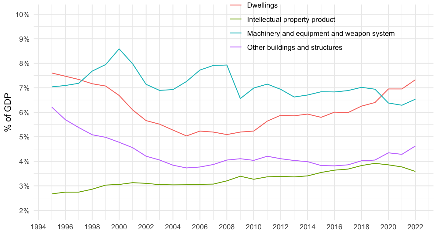
Detailed Components
Code
SNA_TABLE8A %>%
  filter(ACTIVITY == "VTOT",
         MEASURE == "C",
         TRANSACT %in% c("P51N11131A", "P51N1113IA", "P51N1113OA"),
         LOCATION == "DEU") %>%
  left_join(SNA_TABLE8A_var$TRANSACT, by = "TRANSACT") %>%
  left_join(B1_GE_C, by = c("LOCATION", "obsTime")) %>%
  year_to_date %>%
  ggplot + theme_minimal() + ylab("% of GDP") + xlab("") +
  geom_line(aes(x = date, y = obsValue / B1_GE_C, color = Transact)) +
  scale_y_continuous(breaks = 0.01*seq(0, 1300, 1),
                     labels = scales::percent_format(accuracy = 1)) +
  scale_x_date(breaks = seq(1920, 2100, 2) %>% paste0("-01-01") %>% as.Date,
               labels = date_format("%Y")) +

  theme(legend.position = c(0.6, 0.6),
        legend.title = element_blank())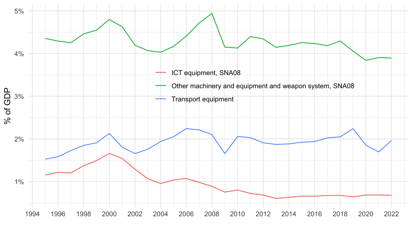
Inventories
Code
SNA_TABLE8A %>%
  filter(ACTIVITY == "VTOT",
         MEASURE == "C",
         TRANSACT %in% c("P52A", "P52_P53A", "P53A"),
         LOCATION == "DEU") %>%
  left_join(SNA_TABLE8A_var$TRANSACT, by = "TRANSACT") %>%
  left_join(B1_GE_C, by = c("LOCATION", "obsTime")) %>%
  year_to_date %>%
  ggplot + theme_minimal() + ylab("% of GDP") + xlab("") +
  geom_line(aes(x = date, y = obsValue / B1_GE_C, color = Transact)) +
  scale_y_continuous(breaks = 0.01*seq(-1, 1300, .5),
                     labels = scales::percent_format(accuracy = .1)) +
  scale_x_date(breaks = seq(1920, 2100, 2) %>% paste0("-01-01") %>% as.Date,
               labels = date_format("%Y")) +

  theme(legend.position = c(0.4, 0.2),
        legend.title = element_blank())
France
Main Components
Code
SNA_TABLE8A %>%
  filter(ACTIVITY == "VTOT",
         MEASURE == "C",
         TRANSACT %in% c("P51N1111A", "P51N1112A", "P51N1113A", "P51N112A"),
         LOCATION == "FRA") %>%
  left_join(SNA_TABLE8A_var$TRANSACT, by = "TRANSACT") %>%
  left_join(B1_GE_C, by = c("LOCATION", "obsTime")) %>%
  year_to_date %>%
  ggplot + theme_minimal() + ylab("% of GDP") + xlab("") +
  geom_line(aes(x = date, y = obsValue / B1_GE_C, color = Transact)) +
  scale_y_continuous(breaks = 0.01*seq(0, 1300, 1),
                     labels = scales::percent_format(accuracy = 1),
                     limits = c(0.02, 0.1)) +
  scale_x_date(breaks = seq(1920, 2100, 2) %>% paste0("-01-01") %>% as.Date,
               labels = date_format("%Y")) +

  theme(legend.position = c(0.7, 0.9),
        legend.title = element_blank())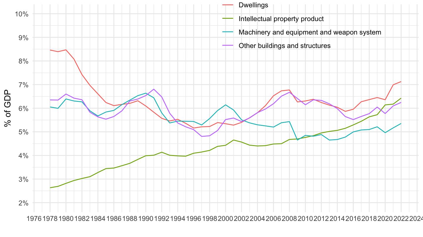
Detailed Components
Code
SNA_TABLE8A %>%
  filter(ACTIVITY == "VTOT",
         MEASURE == "C",
         TRANSACT %in% c("P51N11131A", "P51N1113IA", "P51N1113OA"),
         LOCATION == "FRA") %>%
  left_join(SNA_TABLE8A_var$TRANSACT, by = "TRANSACT") %>%
  left_join(B1_GE_C, by = c("LOCATION", "obsTime")) %>%
  year_to_date %>%
  ggplot + theme_minimal() + ylab("% of GDP") + xlab("") +
  geom_line(aes(x = date, y = obsValue / B1_GE_C, color = Transact)) +
  scale_y_continuous(breaks = 0.01*seq(0, 1300, 1),
                     labels = scales::percent_format(accuracy = 1)) +
  scale_x_date(breaks = seq(1920, 2100, 2) %>% paste0("-01-01") %>% as.Date,
               labels = date_format("%Y")) +

  theme(legend.position = c(0.6, 0.6),
        legend.title = element_blank())
Inventories
Code
SNA_TABLE8A %>%
  filter(ACTIVITY == "VTOT",
         MEASURE == "C",
         TRANSACT %in% c("P52A", "P52_P53A", "P53A"),
         LOCATION == "FRA") %>%
  left_join(SNA_TABLE8A_var$TRANSACT, by = "TRANSACT") %>%
  left_join(B1_GE_C, by = c("LOCATION", "obsTime")) %>%
  year_to_date %>%
  ggplot + theme_minimal() + ylab("% of GDP") + xlab("") +
  geom_line(aes(x = date, y = obsValue / B1_GE_C, color = Transact)) +
  scale_y_continuous(breaks = 0.01*seq(-1, 1300, .5),
                     labels = scales::percent_format(accuracy = .1)) +
  scale_x_date(breaks = seq(1920, 2100, 2) %>% paste0("-01-01") %>% as.Date,
               labels = date_format("%Y")) +

  theme(legend.position = c(0.4, 0.2),
        legend.title = element_blank())
Spain
Main Components
Code
SNA_TABLE8A %>%
  filter(ACTIVITY == "VTOT",
         MEASURE == "C",
         TRANSACT %in% c("P51N1111A", "P51N1112A", "P51N1113A", "P51N112A"),
         LOCATION == "ESP") %>%
  left_join(SNA_TABLE8A_var$TRANSACT, by = "TRANSACT") %>%
  left_join(B1_GE_C, by = c("LOCATION", "obsTime")) %>%
  year_to_date %>%
  ggplot + theme_minimal() + ylab("% of GDP") + xlab("") +
  geom_line(aes(x = date, y = obsValue / B1_GE_C, color = Transact)) +
  scale_y_continuous(breaks = 0.01*seq(0, 1300, 1),
                     labels = scales::percent_format(accuracy = 1)) +
  scale_x_date(breaks = seq(1920, 2100, 2) %>% paste0("-01-01") %>% as.Date,
               labels = date_format("%Y")) +

  theme(legend.position = c(0.78, 0.9),
        legend.title = element_blank())
Detailed Components
Code
SNA_TABLE8A %>%
  filter(ACTIVITY == "VTOT",
         MEASURE == "C",
         TRANSACT %in% c("P51N11131A", "P51N1113IA", "P51N1113OA"),
         LOCATION == "ESP") %>%
  left_join(SNA_TABLE8A_var$TRANSACT, by = "TRANSACT") %>%
  left_join(B1_GE_C, by = c("LOCATION", "obsTime")) %>%
  year_to_date %>%
  ggplot + theme_minimal() + ylab("% of GDP") + xlab("") +
  geom_line(aes(x = date, y = obsValue / B1_GE_C, color = Transact)) +
  scale_y_continuous(breaks = 0.01*seq(0, 1300, 1),
                     labels = scales::percent_format(accuracy = 1)) +
  scale_x_date(breaks = seq(1920, 2100, 2) %>% paste0("-01-01") %>% as.Date,
               labels = date_format("%Y")) +

  theme(legend.position = c(0.6, 0.6),
        legend.title = element_blank())
Inventories
Code
SNA_TABLE8A %>%
  filter(ACTIVITY == "VTOT",
         MEASURE == "C",
         TRANSACT %in% c("P52A", "P52_P53A", "P53A"),
         LOCATION == "ESP") %>%
  left_join(SNA_TABLE8A_var$TRANSACT, by = "TRANSACT") %>%
  left_join(B1_GE_C, by = c("LOCATION", "obsTime")) %>%
  year_to_date %>%
  ggplot + theme_minimal() + ylab("% of GDP") + xlab("") +
  geom_line(aes(x = date, y = obsValue / B1_GE_C, color = Transact)) +
  scale_y_continuous(breaks = 0.01*seq(-1, 1300, .1),
                     labels = scales::percent_format(accuracy = .1)) +
  scale_x_date(breaks = seq(1920, 2100, 2) %>% paste0("-01-01") %>% as.Date,
               labels = date_format("%Y")) +

  theme(legend.position = c(0.4, 0.2),
        legend.title = element_blank())
United States
Main Components
Code
SNA_TABLE8A %>%
  filter(ACTIVITY == "VTOT",
         MEASURE == "C",
         TRANSACT %in% c("P51N1111A", "P51N1112A", "P51N1113A", "P51N112A"),
         LOCATION == "USA") %>%
  left_join(SNA_TABLE8A_var$TRANSACT, by = "TRANSACT") %>%
  left_join(B1_GE_C, by = c("LOCATION", "obsTime")) %>%
  year_to_date %>%
  ggplot + theme_minimal() + ylab("% of GDP") + xlab("") +
  geom_line(aes(x = date, y = obsValue / B1_GE_C, color = Transact)) +
  scale_y_continuous(breaks = 0.01*seq(0, 1300, 1),
                     labels = scales::percent_format(accuracy = 1)) +
  scale_x_date(breaks = seq(1920, 2100, 2) %>% paste0("-01-01") %>% as.Date,
               labels = date_format("%Y")) +

  theme(legend.position = c(0.78, 0.9),
        legend.title = element_blank())
Detailed Components
Code
SNA_TABLE8A %>%
  filter(ACTIVITY == "VTOT",
         MEASURE == "C",
         TRANSACT %in% c("P51N11131A", "P51N1113IA", "P51N1113OA"),
         LOCATION == "USA") %>%
  left_join(SNA_TABLE8A_var$TRANSACT, by = "TRANSACT") %>%
  left_join(B1_GE_C, by = c("LOCATION", "obsTime")) %>%
  year_to_date %>%
  ggplot + theme_minimal() + ylab("% of GDP") + xlab("") +
  geom_line(aes(x = date, y = obsValue / B1_GE_C, color = Transact)) +
  scale_y_continuous(breaks = 0.01*seq(0, 1300, 1),
                     labels = scales::percent_format(accuracy = 1)) +
  scale_x_date(breaks = seq(1920, 2100, 2) %>% paste0("-01-01") %>% as.Date,
               labels = date_format("%Y")) +

  theme(legend.position = c(0.6, 0.6),
        legend.title = element_blank())
United Kingdom
Main Components
Code
SNA_TABLE8A %>%
  filter(ACTIVITY == "VTOT",
         MEASURE == "C",
         TRANSACT %in% c("P51N1111A", "P51N1112A", "P51N1113A", "P51N112A"),
         LOCATION == "GBR") %>%
  left_join(SNA_TABLE8A_var$TRANSACT, by = "TRANSACT") %>%
  left_join(B1_GE_C, by = c("LOCATION", "obsTime")) %>%
  year_to_date %>%
  ggplot + theme_minimal() + ylab("% of GDP") + xlab("") +
  geom_line(aes(x = date, y = obsValue / B1_GE_C, color = Transact)) +
  scale_y_continuous(breaks = 0.01*seq(0, 1300, 1),
                     labels = scales::percent_format(accuracy = 1)) +
  scale_x_date(breaks = seq(1920, 2100, 2) %>% paste0("-01-01") %>% as.Date,
               labels = date_format("%Y")) +

  theme(legend.position = c(0.78, 0.9),
        legend.title = element_blank())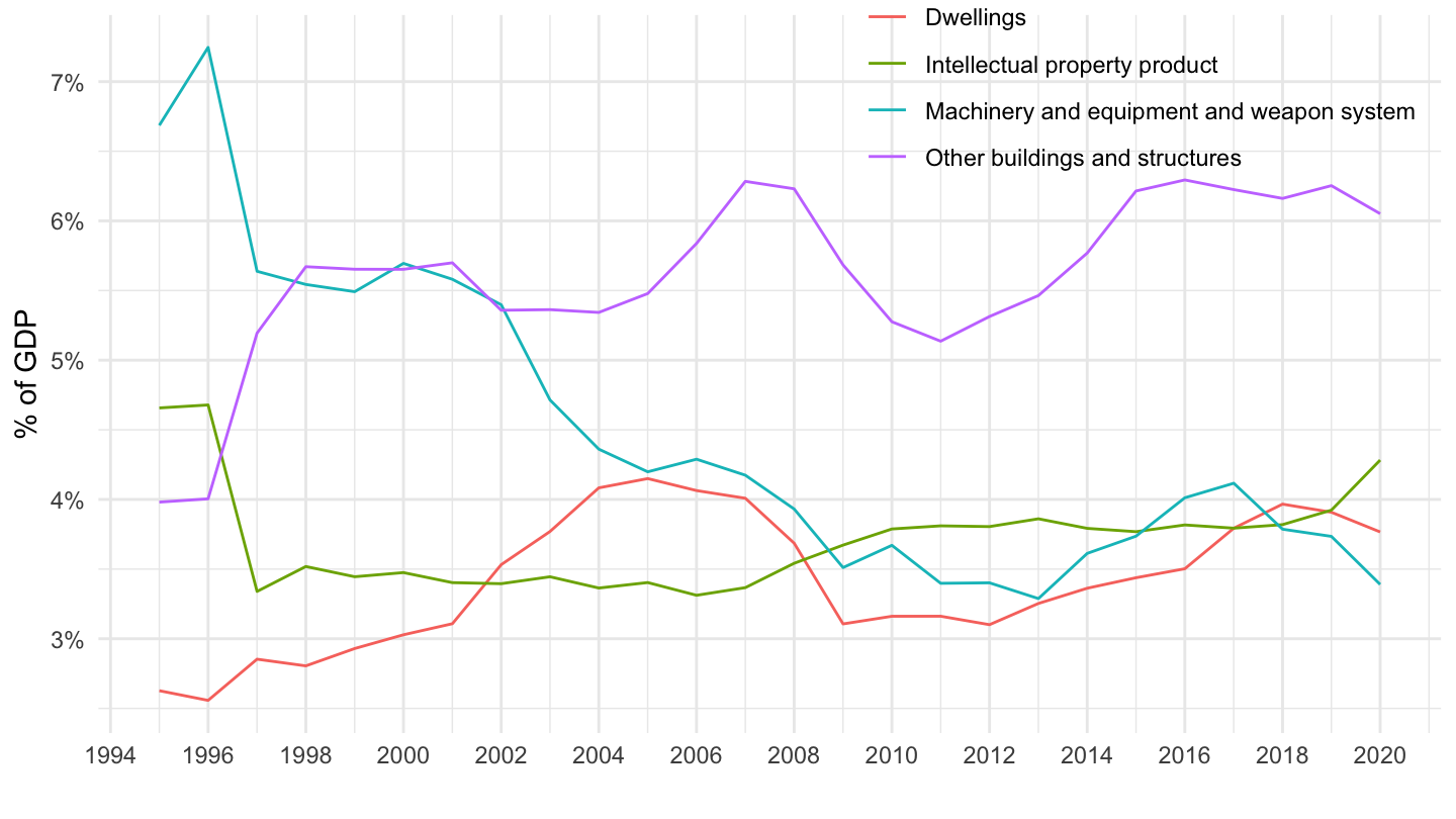
Detailed Components
Code
SNA_TABLE8A %>%
  filter(ACTIVITY == "VTOT",
         MEASURE == "C",
         TRANSACT %in% c("P51N11131A", "P51N1113IA", "P51N1113OA"),
         LOCATION == "GBR") %>%
  left_join(SNA_TABLE8A_var$TRANSACT, by = "TRANSACT") %>%
  left_join(B1_GE_C, by = c("LOCATION", "obsTime")) %>%
  year_to_date %>%
  ggplot + theme_minimal() + ylab("% of GDP") + xlab("") +
  geom_line(aes(x = date, y = obsValue / B1_GE_C, color = Transact)) +
  scale_y_continuous(breaks = 0.01*seq(0, 1300, 1),
                     labels = scales::percent_format(accuracy = 1)) +
  scale_x_date(breaks = seq(1920, 2100, 2) %>% paste0("-01-01") %>% as.Date,
               labels = date_format("%Y")) +

  theme(legend.position = c(0.6, 0.6),
        legend.title = element_blank())
Greece
Main Components
Code
SNA_TABLE8A %>%
  filter(ACTIVITY == "VTOT",
         MEASURE == "C",
         TRANSACT %in% c("P51N1111A", "P51N1112A", "P51N1113A", "P51N112A"),
         LOCATION == "GRC") %>%
  left_join(SNA_TABLE8A_var$TRANSACT, by = "TRANSACT") %>%
  left_join(B1_GE_C, by = c("LOCATION", "obsTime")) %>%
  year_to_date %>%
  ggplot + theme_minimal() + ylab("% of GDP") + xlab("") +
  geom_line(aes(x = date, y = obsValue / B1_GE_C, color = Transact)) +
  scale_y_continuous(breaks = 0.01*seq(0, 1300, 1),
                     labels = scales::percent_format(accuracy = 1)) +
  scale_x_date(breaks = seq(1920, 2100, 2) %>% paste0("-01-01") %>% as.Date,
               labels = date_format("%Y")) +

  theme(legend.position = c(0.78, 0.9),
        legend.title = element_blank())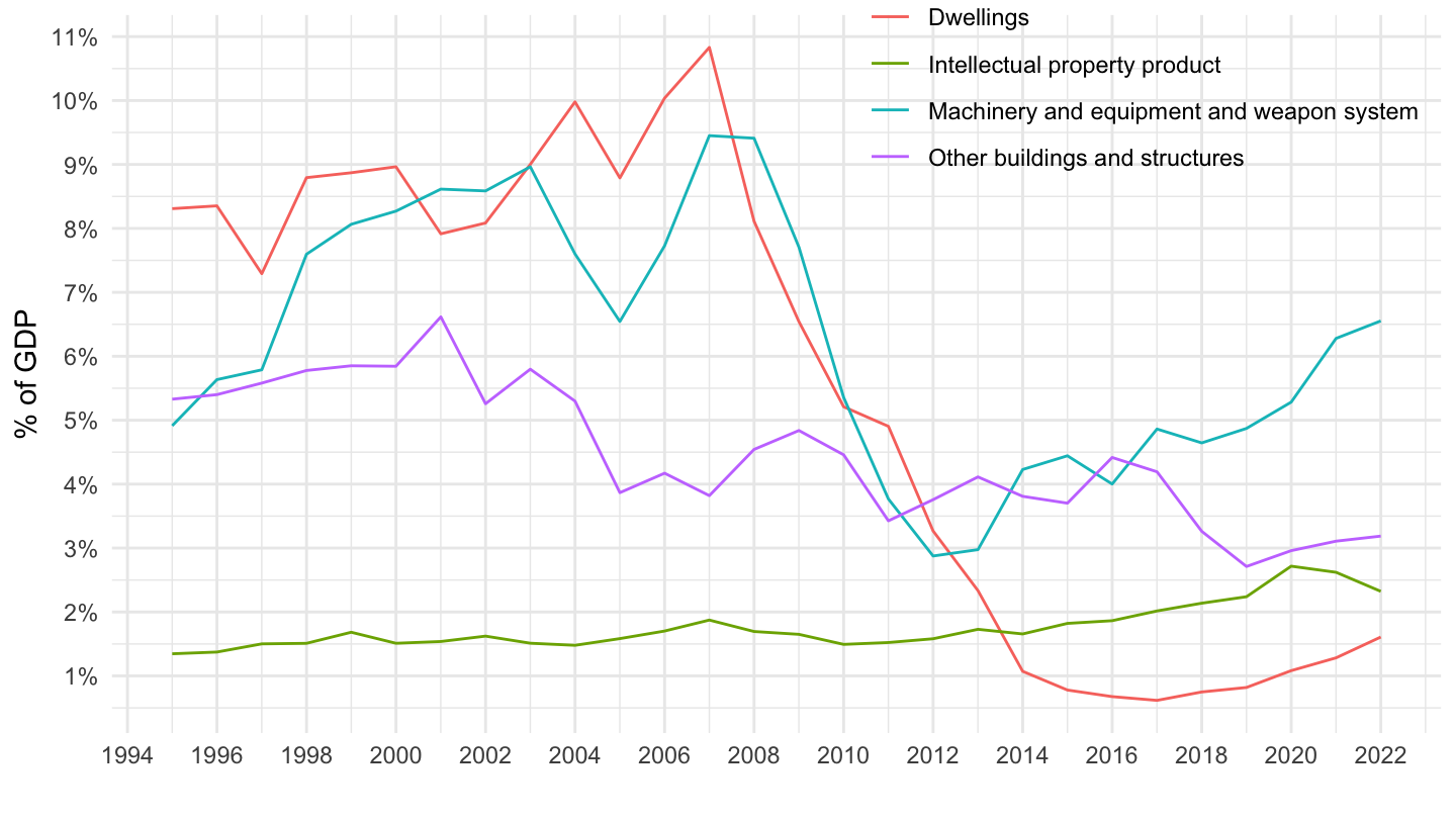
Detailed Components
Code
SNA_TABLE8A %>%
  filter(ACTIVITY == "VTOT",
         MEASURE == "C",
         TRANSACT %in% c("P51N11131A", "P51N1113IA", "P51N1113OA"),
         LOCATION == "GRC") %>%
  left_join(SNA_TABLE8A_var$TRANSACT, by = "TRANSACT") %>%
  left_join(B1_GE_C, by = c("LOCATION", "obsTime")) %>%
  year_to_date %>%
  ggplot + theme_minimal() + ylab("% of GDP") + xlab("") +
  geom_line(aes(x = date, y = obsValue / B1_GE_C, color = Transact)) +
  scale_y_continuous(breaks = 0.01*seq(0, 1300, 1),
                     labels = scales::percent_format(accuracy = 1)) +
  scale_x_date(breaks = seq(1920, 2100, 2) %>% paste0("-01-01") %>% as.Date,
               labels = date_format("%Y")) +

  theme(legend.position = c(0.6, 0.6),
        legend.title = element_blank())
Sweden
Main Components
Code
SNA_TABLE8A %>%
  filter(ACTIVITY == "VTOT",
         MEASURE == "C",
         TRANSACT %in% c("P51N1111A", "P51N1112A", "P51N1113A", "P51N112A"),
         LOCATION == "SWE") %>%
  left_join(SNA_TABLE8A_var$TRANSACT, by = "TRANSACT") %>%
  left_join(B1_GE_C, by = c("LOCATION", "obsTime")) %>%
  year_to_date %>%
  ggplot + theme_minimal() + ylab("% of GDP") + xlab("") +
  geom_line(aes(x = date, y = obsValue / B1_GE_C, color = Transact)) +
  scale_y_continuous(breaks = 0.01*seq(0, 1300, 1),
                     labels = scales::percent_format(accuracy = 1)) +
  scale_x_date(breaks = seq(1920, 2100, 2) %>% paste0("-01-01") %>% as.Date,
               labels = date_format("%Y")) +

  theme(legend.position = c(0.78, 0.9),
        legend.title = element_blank())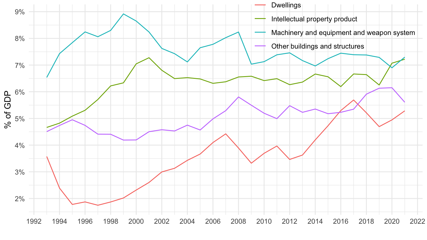
Detailed Components
Code
SNA_TABLE8A %>%
  filter(ACTIVITY == "VTOT",
         MEASURE == "C",
         TRANSACT %in% c("P51N11131A", "P51N1113IA", "P51N1113OA"),
         LOCATION == "SWE") %>%
  left_join(SNA_TABLE8A_var$TRANSACT, by = "TRANSACT") %>%
  left_join(B1_GE_C, by = c("LOCATION", "obsTime")) %>%
  year_to_date %>%
  ggplot + theme_minimal() + ylab("% of GDP") + xlab("") +
  geom_line(aes(x = date, y = obsValue / B1_GE_C, color = Transact)) +
  scale_y_continuous(breaks = 0.01*seq(0, 1300, 1),
                     labels = scales::percent_format(accuracy = 1)) +
  scale_x_date(breaks = seq(1920, 2100, 2) %>% paste0("-01-01") %>% as.Date,
               labels = date_format("%Y")) +

  theme(legend.position = c(0.6, 0.6),
        legend.title = element_blank())
SNA_TABLE8A_ex1
png

Code
Code
SNA_TABLE8A %>%
  filter(ACTIVITY == "VTOT",
         MEASURE == "C",
         LOCATION %in% c("USA", "FRA", "DEU")) %>%
  left_join(SNA_TABLE8A_var$TRANSACT, by = "TRANSACT") %>%
  left_join(SNA_TABLE8A_var$LOCATION, by = "LOCATION") %>%
  rename(`Type of Fixed Asset` = Transact) %>%
  rename(Country = Location) %>%
  filter(obsTime == 2016) %>%
  select(TRANSACT, `Type of Fixed Asset`, Country, obsValue) %>%
  arrange(TRANSACT) %>%
  group_by(Country) %>%
  mutate(obsValue = ifelse(!is.na(obsValue), paste0(round(100*obsValue / obsValue[1], digits = 1), "%"), "")) %>%
  spread(Country, obsValue) %>%
  mutate_at(vars(-1, -2), funs(ifelse(is.na(.), "", .))) %>%
{if (is_html_output() | is_latex_output()) print_table(.) else .}| TRANSACT | Type of Fixed Asset | France | Germany | United States |
|---|---|---|---|---|
| B1_GE | Gross domestic product (expenditure approach) | 100% | 100% | 100% |
| P51A | Gross fixed capital formation | 21.8% | 20.3% | 20% |
| P51N1111A | Dwellings | 6% | 6% | 3.7% |
| P51N1112A | Other buildings and structures | 5.5% | 3.8% | 4.4% |
| P51N11131A | Transport equipment | 1.6% | 1.9% | 1.6% |
| P51N111321A | Computer hardware | 0.2% | 0.4% | 0.6% |
| P51N111322A | Telecommunications equipment | 0.2% | 0.3% | 0.6% |
| P51N1113A | Machinery and equipment and weapon system | 5% | 6.8% | 6.5% |
| P51N1113IA | ICT equipment, SNA08 | 0.5% | 0.7% | 1.2% |
| P51N1113OA | Other machinery and equipment and weapon system, SNA08 | 2.9% | 4.2% | 3.7% |
| P51N1114A | Cultivated biological resources | 0.1% | 0% | |
| P51N111XA | Total construction | 11.5% | 9.8% | 8.1% |
| P51N11221A | Computer software | 2% | ||
| P51N1122A | Computer software and databases | 2.9% | 0.7% | 2% |
| P51N1123A | Entertainment, literary and artistic originals | 0.4% | ||
| P51N1124A | Research and development | 2.2% | 2.7% | 2.9% |
| P51N112A | Intellectual property product | 5.3% | 3.6% | 5.4% |
| P52_P53A | Changes in inventories and acquisition less disposals of valuables | 0.8% | -0.3% | |
| P52A | Changes in inventories | 0.8% | -0.4% | |
| P53A | Acquisition less disposals of valuables | 0% | 0.1% | |
| P5A | Gross capital formation | 22.6% | 20% |