Industrial production
Data - OECD
Info
Last observation: Monthly: 2026-06 (N = 14) · Quarterly: 2026-Q1 (N = 430) · Annual: 2025 (N = 468)
First observation: Monthly: 1919-01 (N = 4) · Quarterly: 1919-Q1 (N = 4) · Annual: 1919 (N = 4)
Last data update: 24 jul 2026, 02:52. Last compile: 24 jul 2026, 03:52
Structure
Industrial Production
Etats-Unis vs Zone euro
All
Code
INDSERV %>%
  filter(MEASURE == "PRVM",
         ACTIVITY == "C",
         FREQ == "M",
         ADJUSTMENT == "Y",
         REF_AREA %in% c("USA", "EA20")) %>%

  month_to_date %>%
  group_by(date) %>%
  group_by(Ref_area) %>%
  arrange(date) %>%
  mutate(obsValue = 100*obsValue/obsValue[1]) %>%
  mutate(Ref_area = ifelse(REF_AREA == "EA20", "Europe", Ref_area)) %>%
  left_join(colors, by = c("Ref_area" = "country")) %>%
  mutate(Ref_area2 = ifelse(REF_AREA == "EA20", "Eurozone", Ref_area),
         color = ifelse(REF_AREA == "USA", color2, color)) %>%
  ggplot(.) + geom_line(aes(x = date, y = obsValue, color = color)) +
  scale_color_identity() + add_2flags +
  theme_minimal() + xlab("") + ylab("Production manufacturière (Janv. 1980 = 100)") +
  scale_x_date(breaks = c(seq(1970, 2100, 5),seq(1980, 2100, 5)) %>% paste0("-01-01") %>% as.Date,
               labels = date_format("%Y")) +
  scale_y_log10(breaks = seq(-10, 300, 5),
                     labels = dollar_format(accuracy = 1, prefix = "")) +
  theme(legend.position = c(0.2, 0.80),
        legend.title = element_blank()) +
  labs(caption = "Source: OCDE")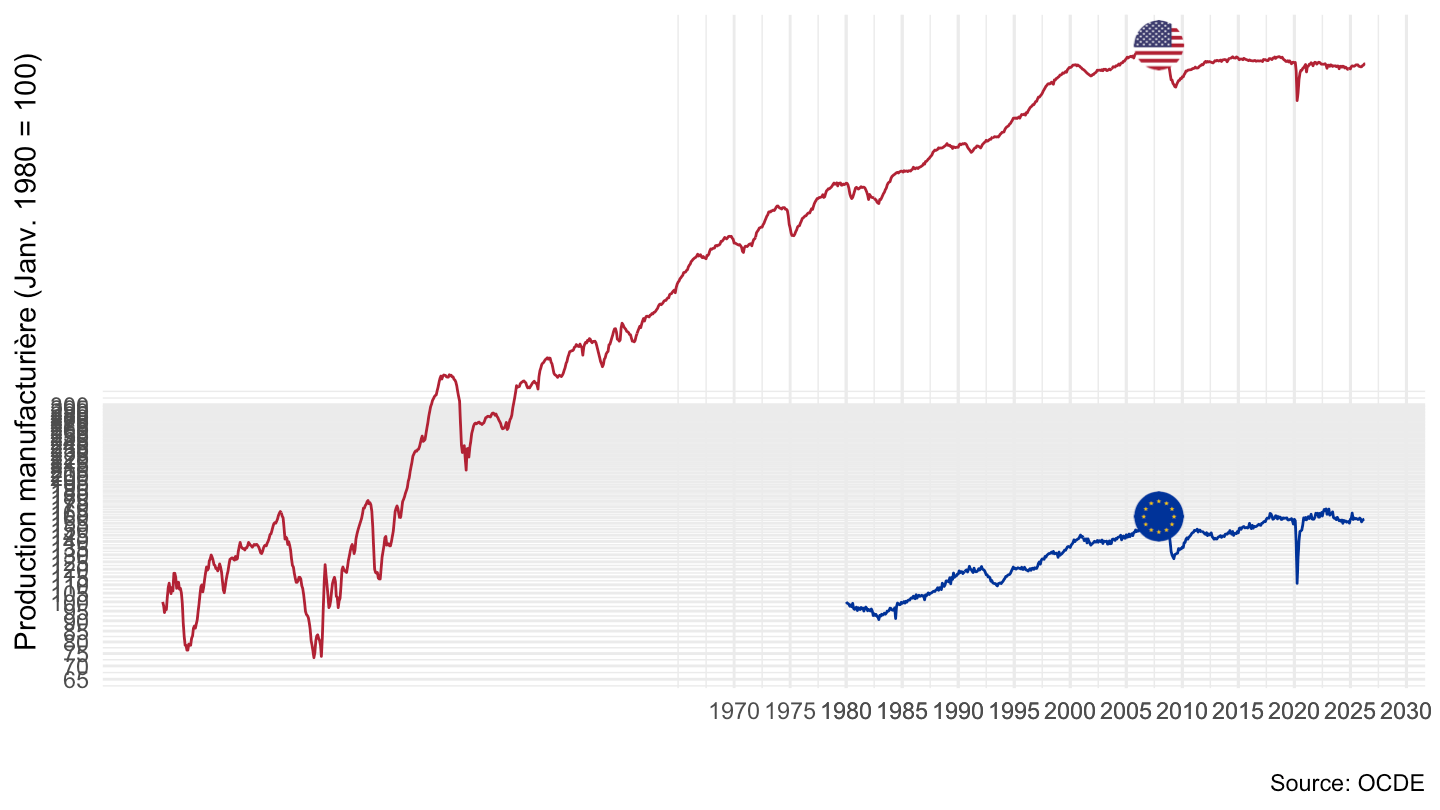
Etats-Unis vs Zone euro
All
Code
INDSERV %>%
  filter(MEASURE == "PRVM",
         ACTIVITY == "C",
         FREQ == "M",
         ADJUSTMENT == "Y",
         REF_AREA %in% c("USA", "EA20")) %>%

  month_to_date %>%
  group_by(date) %>%
  group_by(Ref_area) %>%
  arrange(date) %>%
  mutate(obsValue = 100*obsValue/obsValue[1]) %>%
  mutate(Ref_area = ifelse(REF_AREA == "EA20", "Europe", Ref_area)) %>%
  left_join(colors, by = c("Ref_area" = "country")) %>%
  mutate(Ref_area2 = ifelse(REF_AREA == "EA20", "Eurozone", Ref_area),
         color = ifelse(REF_AREA == "USA", color2, color)) %>%
  ggplot(.) + geom_line(aes(x = date, y = obsValue, color = color)) +
  scale_color_identity() + add_2flags +
  theme_minimal() + xlab("") + ylab("Production manufacturière (Janv. 1980 = 100)") +
  scale_x_date(breaks = c(seq(1970, 2100, 5),seq(1980, 2100, 5)) %>% paste0("-01-01") %>% as.Date,
               labels = date_format("%Y")) +
  scale_y_log10(breaks = seq(-10, 300, 5),
                     labels = dollar_format(accuracy = 1, prefix = "")) +
  theme(legend.position = c(0.2, 0.80),
        legend.title = element_blank()) +
  geom_rect(data = nber_recessions %>%
              filter(Peak > as.Date("1980-01-01")),
            aes(xmin = Peak, xmax = Trough, ymin = 0, ymax = +Inf),
            fill = '#B22234', alpha = 0.1)  +
  geom_rect(data = cepr_recessions %>%
              filter(Peak > as.Date("1980-01-01")),
            aes(xmin = Peak, xmax = Trough, ymin = 0, ymax = +Inf),
            fill = '#003399', alpha = 0.1) +
  labs(caption = "Source: OCDE")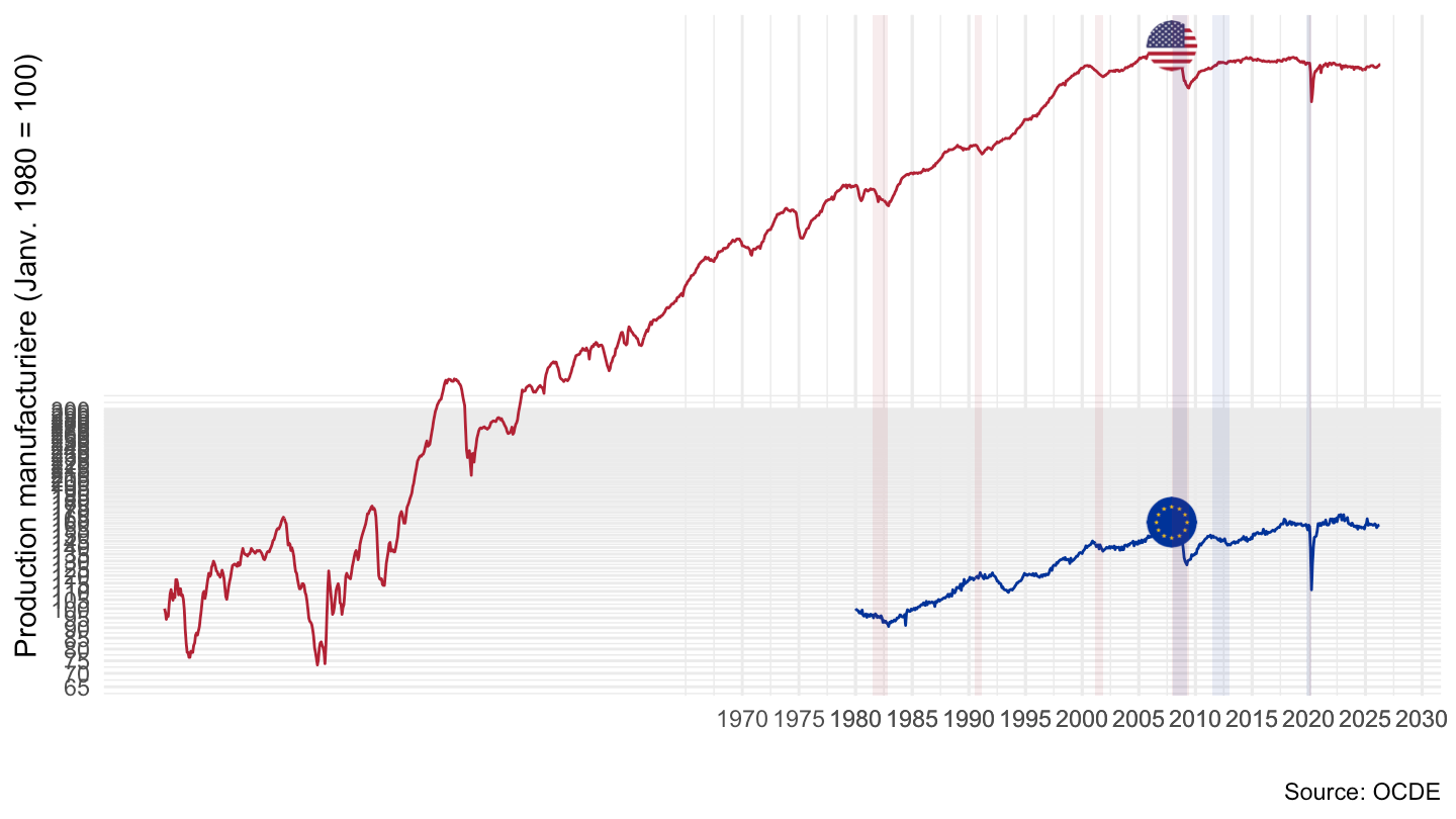
1999-
Code
plot <- INDSERV %>%
  filter(MEASURE == "PRVM",
         ACTIVITY == "C",
         FREQ == "M",
         ADJUSTMENT == "Y",
         REF_AREA %in% c("USA", "EA20")) %>%

  month_to_date %>%
  filter(date >= as.Date("1999-01-01")) %>%
  group_by(Ref_area) %>%
  arrange(date) %>%
  mutate(obsValue = 100*obsValue/obsValue[1]) %>%
  mutate(Ref_area = ifelse(REF_AREA == "EA20", "Zone euro", Ref_area)) %>%
  ggplot(.) + geom_line(aes(x = date, y = obsValue, color = Ref_area)) +
  scale_color_manual(values = c("#B22234", "#003399")) +
  theme_minimal() + xlab("") + ylab("Production manufacturière (Janv. 1999 = 100)") +
  scale_x_date(breaks = c(seq(1999, 2100, 5),seq(1997, 2100, 5)) %>% paste0("-01-01") %>% as.Date,
               labels = date_format("%Y")) +
  scale_y_log10(breaks = seq(-10, 300, 5),
                     labels = dollar_format(accuracy = 1, prefix = "")) +
  theme(legend.position = c(0.2, 0.80),
        legend.title = element_blank()) +
  geom_rect(data = nber_recessions %>%
              filter(Peak > as.Date("1999-01-01")),
            aes(xmin = Peak, xmax = Trough, ymin = 0, ymax = +Inf),
            fill = '#B22234', alpha = 0.1)  +
  geom_rect(data = cepr_recessions %>%
              filter(Peak > as.Date("1999-01-01")),
            aes(xmin = Peak, xmax = Trough, ymin = 0, ymax = +Inf),
            fill = '#003399', alpha = 0.1) +
  labs(caption = "Source: OCDE")

save(plot, file = "INDSERV_files/figure-html/PRVM-C-USA-EA-1999-1.RData")
plot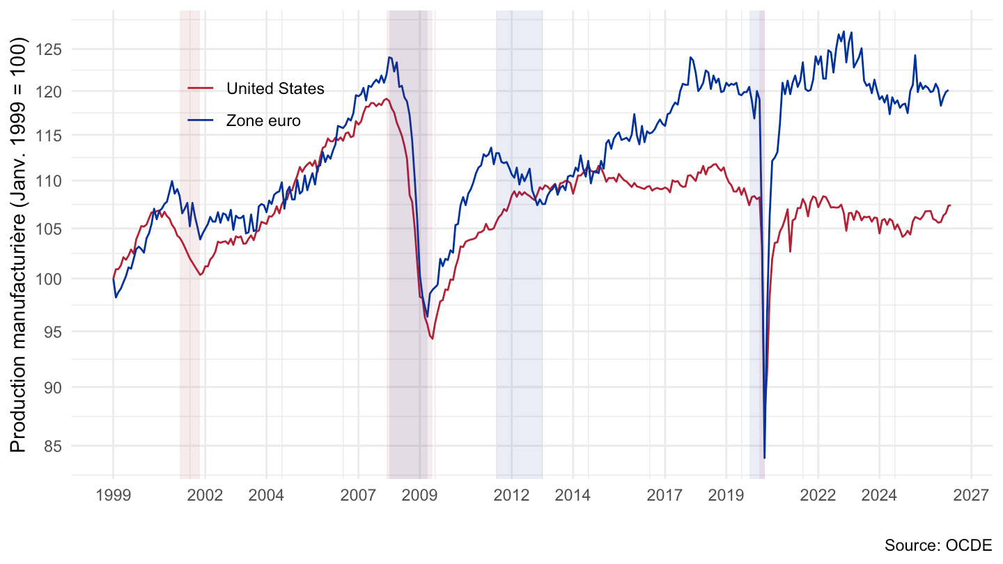
France, Italy, US, Europe, Greece
All
Code
INDSERV %>%
  filter(MEASURE == "PRVM",
         ACTIVITY == "C",
         FREQ == "M",
         ADJUSTMENT == "Y",
         REF_AREA %in% c("USA", "EA20", "ITA", "FRA", "DEU", "GRC")) %>%

  month_to_date %>%
  group_by(date) %>%
  #filter(n() == 6) %>%
  #filter(date >= as.Date("1999-01-01")) %>%
  group_by(Ref_area) %>%
  arrange(date) %>%
  mutate(obsValue = 100*obsValue/obsValue[1]) %>%
  mutate(Ref_area = ifelse(REF_AREA == "EA20", "Europe", Ref_area)) %>%
  left_join(colors, by = c("Ref_area" = "country")) %>%
  mutate(color = ifelse(REF_AREA == "EA20", color2, color)) %>%
  ggplot(.) + geom_line(aes(x = date, y = obsValue, color = color)) +
  theme_minimal() + xlab("") + ylab("Production manufacturière (Janv. 1999 = 100)") +
  scale_color_identity() + add_6flags +
  scale_x_date(breaks = c(seq(1920, 2100, 10)) %>% paste0("-01-01") %>% as.Date,
               labels = date_format("%Y")) +
  scale_y_log10(breaks = seq(100, 10000, 100),
                     labels = dollar_format(accuracy = 1, prefix = "")) +
  theme(legend.position = c(0.2, 0.80),
        legend.title = element_blank())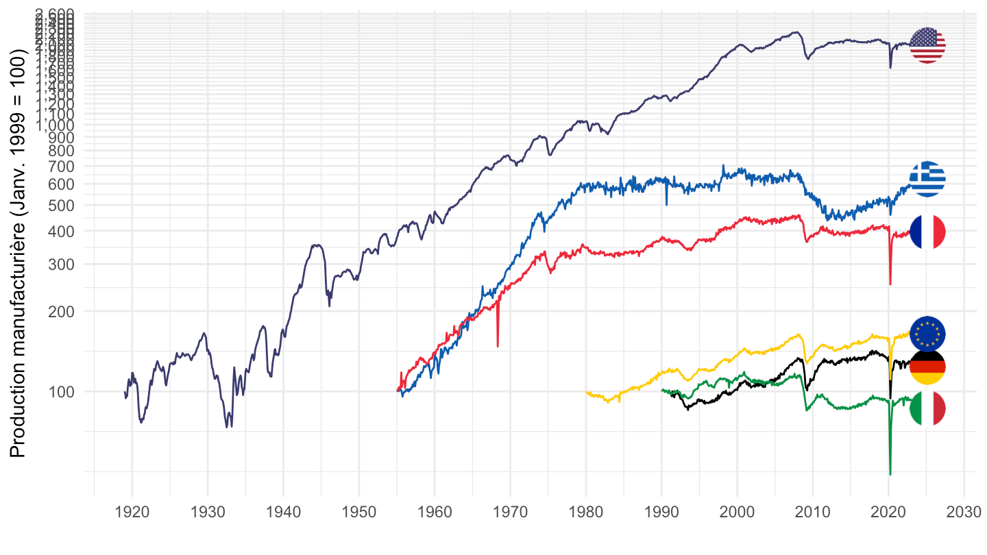
Code
# + labs(caption = "Source: OCDE, calculs de @FrancoisGeerolf")1955-
Code
INDSERV %>%
  filter(MEASURE == "PRVM",
         ACTIVITY == "C",
         FREQ == "M",
         ADJUSTMENT == "Y",
         REF_AREA %in% c("USA", "EA20", "ITA", "FRA", "DEU", "GRC")) %>%

  month_to_date %>%
  group_by(date) %>%
  #filter(n() == 6) %>%
  filter(date >= as.Date("1955-01-01")) %>%
  group_by(Ref_area) %>%
  arrange(date) %>%
  mutate(obsValue = 100*obsValue/obsValue[1]) %>%
  mutate(Ref_area = ifelse(REF_AREA == "EA20", "Europe", Ref_area)) %>%
  left_join(colors, by = c("Ref_area" = "country")) %>%
  mutate(color = ifelse(REF_AREA == "EA20", color2, color)) %>%
  ggplot(.) + geom_line(aes(x = date, y = obsValue, color = color)) +
  theme_minimal() + xlab("") + ylab("Production manufacturière (Janv. 1999 = 100)") +
  scale_color_identity() + add_6flags +
  scale_x_date(breaks = c(seq(1920, 2100, 10)) %>% paste0("-01-01") %>% as.Date,
               labels = date_format("%Y")) +
  scale_y_log10(breaks = seq(100, 10000, 100),
                     labels = dollar_format(accuracy = 1, prefix = "")) +
  theme(legend.position = c(0.2, 0.80),
        legend.title = element_blank())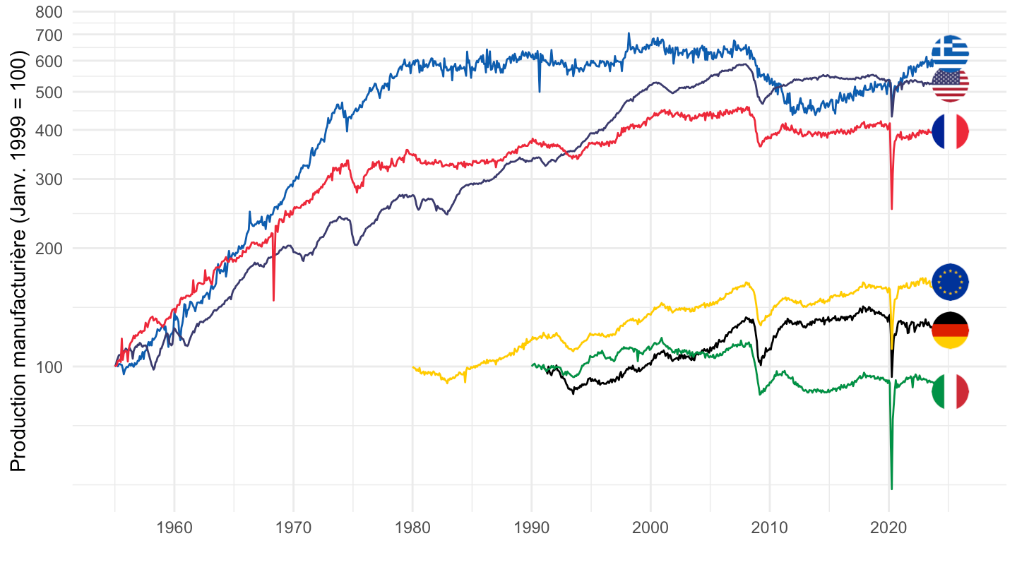
Code
# + labs(caption = "Source: OCDE, calculs de @FrancoisGeerolf")1980-
Code
INDSERV %>%
  filter(MEASURE == "PRVM",
         ACTIVITY == "C",
         FREQ == "M",
         ADJUSTMENT == "Y",
         REF_AREA %in% c("USA", "EA20", "ITA", "FRA", "DEU", "GRC")) %>%

  month_to_date %>%
  group_by(date) %>%
  #filter(n() == 6) %>%
  filter(date >= as.Date("1980-01-01")) %>%
  group_by(Ref_area) %>%
  arrange(date) %>%
  mutate(obsValue = 100*obsValue/obsValue[1]) %>%
  mutate(Ref_area = ifelse(REF_AREA == "EA20", "Europe", Ref_area)) %>%
  left_join(colors, by = c("Ref_area" = "country")) %>%
  mutate(color = ifelse(REF_AREA == "EA20", color2, color)) %>%
  ggplot(.) + geom_line(aes(x = date, y = obsValue, color = color)) +
  theme_minimal() + xlab("") + ylab("Production manufacturière") +
  scale_color_identity() + add_6flags +
  scale_x_date(breaks = c(seq(1920, 2100, 5)) %>% paste0("-01-01") %>% as.Date,
               labels = date_format("%Y")) +
  scale_y_log10(breaks = seq(10, 10000, 10),
                     labels = dollar_format(accuracy = 1, prefix = "")) +
  theme(legend.position = c(0.2, 0.80),
        legend.title = element_blank())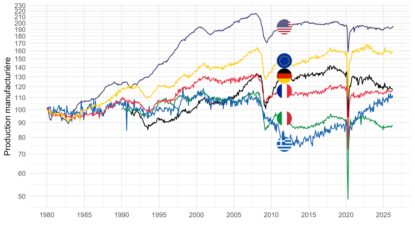
Code
# + labs(caption = "Source: OCDE, calculs de @FrancoisGeerolf")2000-
Code
INDSERV %>%
  filter(MEASURE == "PRVM",
         ACTIVITY == "C",
         FREQ == "M",
         ADJUSTMENT == "Y",
         REF_AREA %in% c("USA", "EA20", "ITA", "FRA", "DEU", "GRC")) %>%

  month_to_date %>%
  group_by(date) %>%
  #filter(n() == 6) %>%
  filter(date >= as.Date("2000-01-01")) %>%
  group_by(Ref_area) %>%
  arrange(date) %>%
  mutate(obsValue = 100*obsValue/obsValue[1]) %>%
  mutate(Ref_area = ifelse(REF_AREA == "EA20", "Europe", Ref_area)) %>%
  left_join(colors, by = c("Ref_area" = "country")) %>%
  mutate(color = ifelse(REF_AREA == "EA20", color2, color)) %>%
  ggplot(.) + geom_line(aes(x = date, y = obsValue, color = color)) +
  theme_minimal() + xlab("") + ylab("Production manufacturière") +
  scale_color_identity() + add_flags +
  scale_x_date(breaks = c(seq(1920, 2100, 5)) %>% paste0("-01-01") %>% as.Date,
               labels = date_format("%Y")) +
  scale_y_log10(breaks = seq(10, 10000, 10),
                     labels = dollar_format(accuracy = 1, prefix = "")) +
  theme(legend.position = c(0.2, 0.80),
        legend.title = element_blank())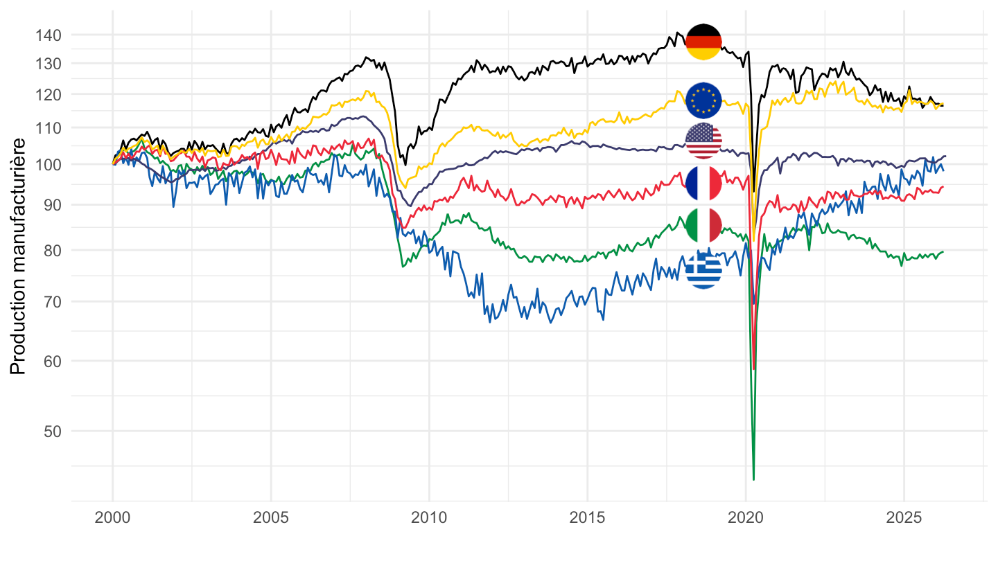
Code
# + labs(caption = "Source: OCDE, calculs de @FrancoisGeerolf")6 observations
Code
INDSERV %>%
  filter(MEASURE == "PRVM",
         ACTIVITY == "C",
         FREQ == "M",
         ADJUSTMENT == "Y",
         REF_AREA %in% c("USA", "EA20", "ITA", "FRA", "DEU", "GRC")) %>%

  month_to_date %>%
  group_by(date) %>%
  #filter(date >= as.Date("1999-01-01")) %>%
  group_by(Ref_area) %>%
  arrange(date) %>%
  mutate(obsValue = 100*obsValue/obsValue[1]) %>%
  mutate(Ref_area = ifelse(REF_AREA == "EA20", "Europe", Ref_area)) %>%
  left_join(colors, by = c("Ref_area" = "country")) %>%
  mutate(color = ifelse(REF_AREA == "EA20", color2, color)) %>%
  ggplot(.) + geom_line(aes(x = date, y = obsValue, color = color)) +
  theme_minimal() + xlab("") + ylab("Production manufacturière (Janv. 1999 = 100)") +
  scale_color_identity() + add_6flags +
  scale_x_date(breaks = c(seq(1979, 2100, 5),seq(1977, 2100, 5)) %>% paste0("-01-01") %>% as.Date,
               labels = date_format("%Y")) +
  scale_y_log10(breaks = seq(-10, 300, 5),
                     labels = dollar_format(accuracy = 1, prefix = "")) +
  theme(legend.position = c(0.2, 0.80),
        legend.title = element_blank())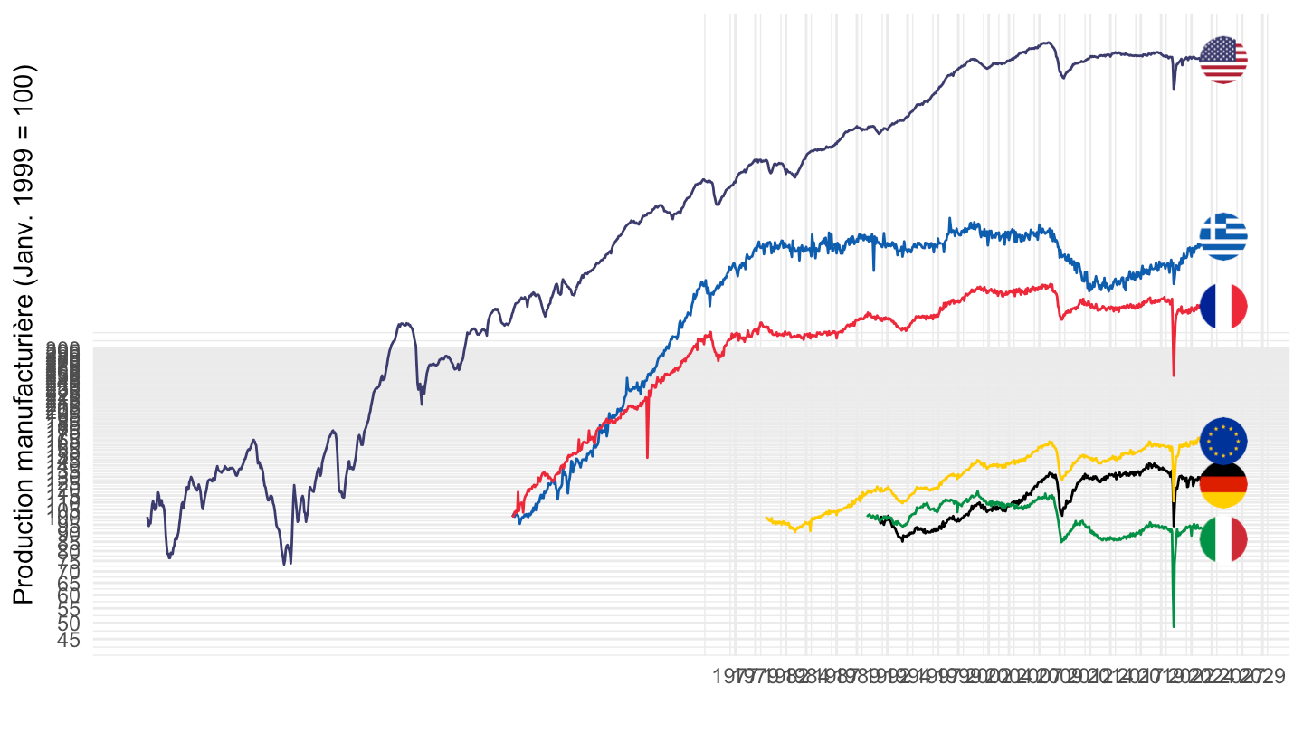
Code
# + labs(caption = "Source: OCDE, calculs de @FrancoisGeerolf")France, Italy, US, Europe
All
Code
INDSERV %>%
  filter(MEASURE == "PRVM",
         ACTIVITY == "C",
         FREQ == "M",
         ADJUSTMENT == "Y",
         REF_AREA %in% c("USA", "EA20", "ITA", "FRA", "DEU")) %>%

  month_to_date %>%
  group_by(date) %>%
  #filter(date >= as.Date("1999-01-01")) %>%
  group_by(Ref_area) %>%
  arrange(date) %>%
  mutate(obsValue = 100*obsValue/obsValue[1]) %>%
  mutate(Ref_area = ifelse(REF_AREA == "EA20", "Europe", Ref_area)) %>%
  left_join(colors, by = c("Ref_area" = "country")) %>%
  mutate(color = ifelse(REF_AREA == "EA20", color2, color)) %>%
  ggplot(.) + geom_line(aes(x = date, y = obsValue, color = color)) +
  theme_minimal() + xlab("") + ylab("Production manufacturière (Janv. 1999 = 100)") +
  scale_color_identity() + add_5flags +
  scale_x_date(breaks = c(seq(1979, 2100, 5),seq(1977, 2100, 5)) %>% paste0("-01-01") %>% as.Date,
               labels = date_format("%Y")) +
  scale_y_log10(breaks = seq(-10, 300, 5),
                     labels = dollar_format(accuracy = 1, prefix = "")) +
  theme(legend.position = c(0.2, 0.80),
        legend.title = element_blank())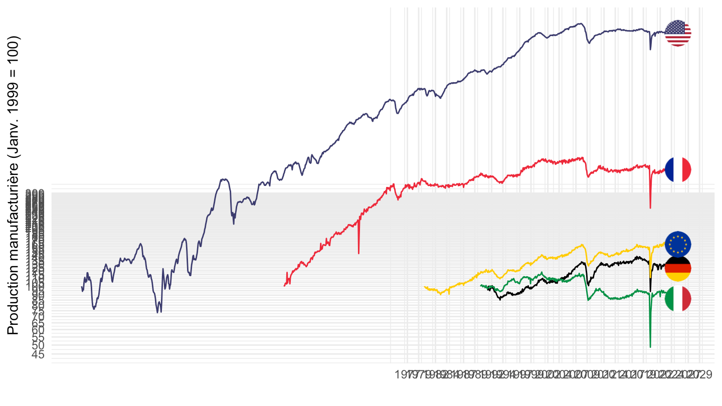
Code
# + labs(caption = "Source: OCDE, calculs de @FrancoisGeerolf")1999-
Code
INDSERV %>%
  filter(MEASURE == "PRVM",
         ACTIVITY == "C",
         FREQ == "M",
         ADJUSTMENT == "Y",
         REF_AREA %in% c("USA", "EA20", "ITA", "FRA", "DEU")) %>%

  month_to_date %>%
  filter(date >= as.Date("1999-01-01")) %>%
  group_by(Ref_area) %>%
  arrange(date) %>%
  mutate(obsValue = 100*obsValue/obsValue[1]) %>%
  mutate(Ref_area = ifelse(REF_AREA == "EA20", "Europe", Ref_area)) %>%
  left_join(colors, by = c("Ref_area" = "country")) %>%
  mutate(color = ifelse(REF_AREA == "EA20", color2, color)) %>%
  ggplot(.) + geom_line(aes(x = date, y = obsValue, color = color)) +
  theme_minimal() + xlab("") + ylab("Production manufacturière (Janv. 1999 = 100)") +
  scale_color_identity() + add_5flags +
  scale_x_date(breaks = c(seq(1999, 2100, 5),seq(1997, 2100, 5)) %>% paste0("-01-01") %>% as.Date,
               labels = date_format("%Y")) +
  scale_y_log10(breaks = seq(-10, 300, 5),
                     labels = dollar_format(accuracy = 1, prefix = "")) +
  theme(legend.position = c(0.2, 0.80),
        legend.title = element_blank())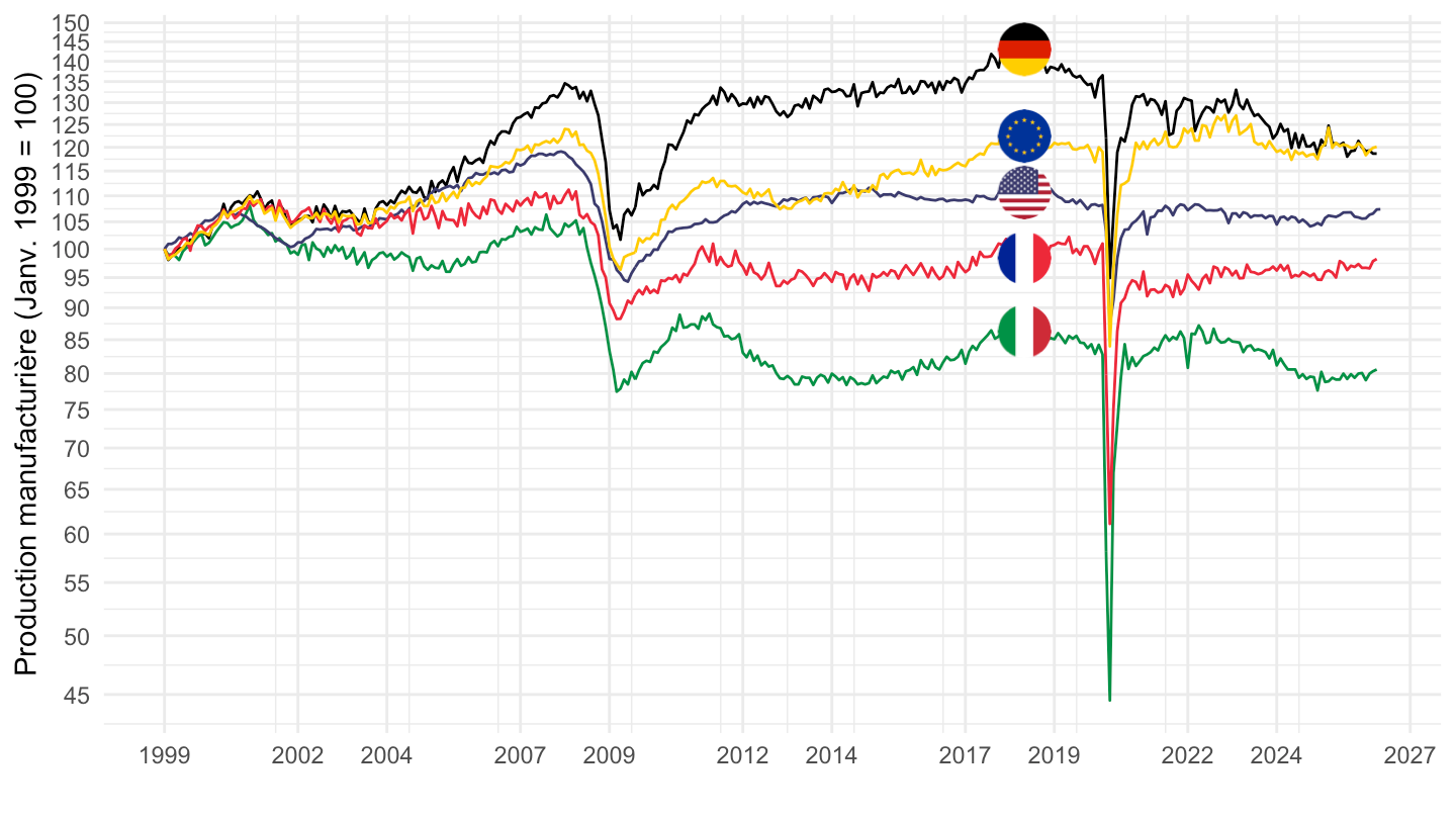
Code
# + labs(caption = "Source: OCDE, calculs de @FrancoisGeerolf")Etats-Unis vs Zone euro VS EU27_2020
All
Code
INDSERV %>%
  filter(MEASURE == "PRVM",
         ACTIVITY == "C",
         FREQ == "M",
         ADJUSTMENT == "Y",
         REF_AREA %in% c("USA", "EA20", "EU27_2020")) %>%

  month_to_date %>%
  group_by(date) %>%
  filter(n() == 3) %>%
  group_by(Ref_area) %>%
  arrange(date) %>%
  mutate(obsValue = 100*obsValue/obsValue[1]) %>%
  mutate(Ref_area = case_when(REF_AREA == "EA20" ~ "Zone euro",
                              REF_AREA == "EU27_2020" ~ "Union Européenne à 27",
                              TRUE ~ Ref_area)) %>%
  mutate(REF_AREA = ifelse(REF_AREA == "EU27_2020", "EU27", REF_AREA)) %>%
  ggplot(.) + geom_line(aes(x = date, y = obsValue, color = Ref_area)) +
  theme_minimal() + xlab("") + ylab("Production manufacturière (Janv. 1999 = 100)") +
  scale_x_date(breaks = seq(1990, 2100, 5) %>% paste0("-01-01") %>% as.Date,
               labels = date_format("%Y")) +
  scale_y_log10(breaks = seq(-10, 300, 5),
                     labels = dollar_format(accuracy = 1, prefix = "")) +
  theme(legend.position = c(0.15, 0.85),
        legend.title = element_blank()) +
  geom_label(data = . %>% filter(date == max(date)), aes(x = date, y = obsValue, label = REF_AREA, color = Ref_area))
1999-
Code
INDSERV %>%
  filter(MEASURE == "PRVM",
         ACTIVITY == "C",
         FREQ == "M",
         ADJUSTMENT == "Y",
         REF_AREA %in% c("USA", "EA20", "EU27_2020")) %>%

  month_to_date %>%
  filter(date >= as.Date("1999-01-01")) %>%
  group_by(Ref_area) %>%
  arrange(date) %>%
  mutate(obsValue = 100*obsValue/obsValue[1]) %>%
  mutate(Ref_area = case_when(REF_AREA == "EA20" ~ "Zone euro",
                              REF_AREA == "EU27_2020" ~ "Union Européenne à 27",
                              TRUE ~ Ref_area)) %>%
  mutate(REF_AREA = ifelse(REF_AREA == "EU27_2020", "EU27", REF_AREA)) %>%
  ggplot(.) + geom_line(aes(x = date, y = obsValue, color = Ref_area)) +
  theme_minimal() + xlab("") + ylab("Production manufacturière (Janv. 1999 = 100)") +
  scale_x_date(breaks = c(seq(2000, 2100, 5),seq(1997, 2100, 5)) %>% paste0("-01-01") %>% as.Date,
               labels = date_format("%Y")) +
  scale_y_log10(breaks = seq(-10, 300, 5),
                     labels = dollar_format(accuracy = 1, prefix = "")) +
  theme(legend.position = c(0.2, 0.80),
        legend.title = element_blank()) +
  geom_label(data = . %>% filter(date == max(date)), aes(x = date, y = obsValue, label = REF_AREA, color = Ref_area))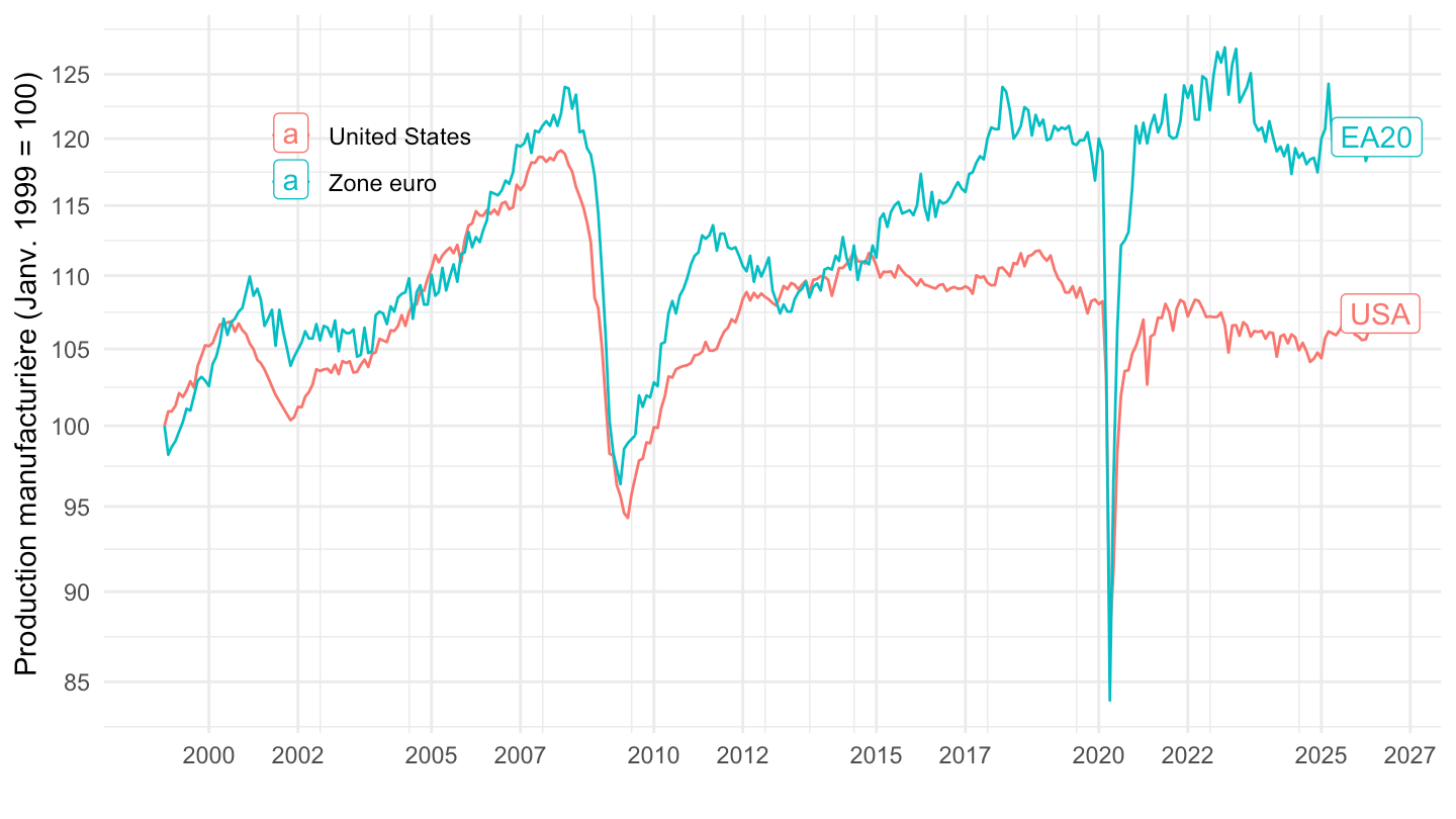
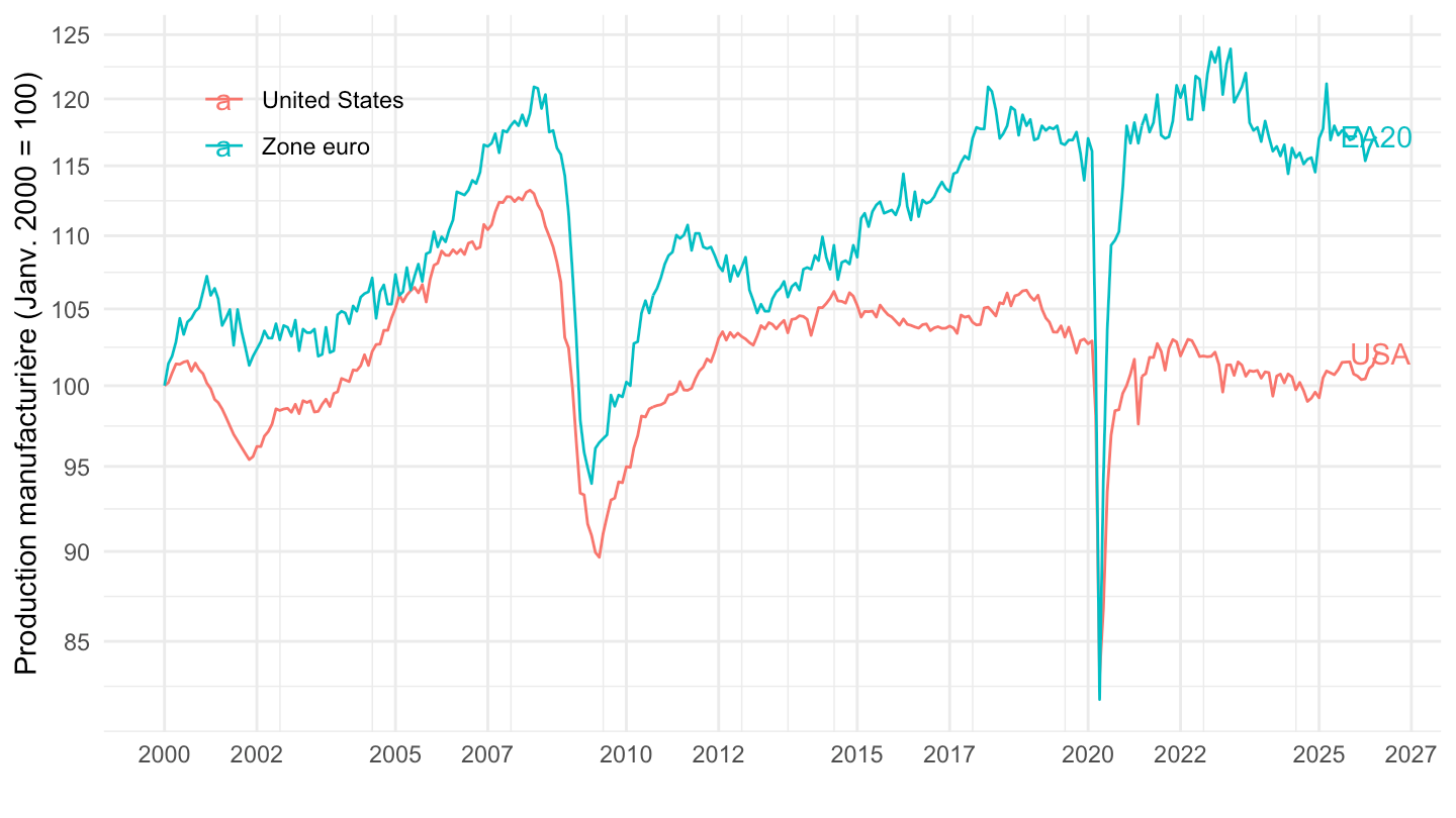
2000-
Code
INDSERV %>%
  filter(MEASURE == "PRVM",
         ACTIVITY == "C",
         FREQ == "M",
         ADJUSTMENT == "Y",
         REF_AREA %in% c("USA", "EA20", "EU27_2020")) %>%

  month_to_date %>%
  filter(date >= as.Date("2000-01-01")) %>%
  group_by(Ref_area) %>%
  arrange(date) %>%
  mutate(obsValue = 100*obsValue/obsValue[1]) %>%
  mutate(Ref_area = case_when(REF_AREA == "EA20" ~ "Zone euro",
                              REF_AREA == "EU27_2020" ~ "Union Européenne à 27",
                              TRUE ~ Ref_area)) %>%
  mutate(REF_AREA = ifelse(REF_AREA == "EU27_2020", "EU27", REF_AREA)) %>%
  ggplot(.) + geom_line(aes(x = date, y = obsValue, color = Ref_area)) +
  theme_minimal() + xlab("") + ylab("Production manufacturière (Janv. 2000 = 100)") +
  scale_x_date(breaks = c(seq(2000, 2100, 5),seq(1997, 2100, 5)) %>% paste0("-01-01") %>% as.Date,
               labels = date_format("%Y")) +
  scale_y_log10(breaks = seq(-10, 300, 5),
                     labels = dollar_format(accuracy = 1, prefix = "")) +
  theme(legend.position = c(0.15, 0.85),
        legend.title = element_blank()) +
  geom_text(data = . %>% filter(date == max(date)), aes(x = date, y = obsValue, label = REF_AREA, color = Ref_area))