Income Distribution Database - IDD
Data - OECD
Info
DOWNLOAD_TIME
| DOWNLOAD_TIME |
|---|
| 2024-04-08 |
Last
| obsTime | Nobs |
|---|---|
| 2022 | 354 |
MEASURE
Code
IDD %>%
  left_join(IDD_var$MEASURE, by = "MEASURE") %>%
  group_by(MEASURE, Measure) %>%
  summarise(Nobs = n()) %>%
  arrange(-Nobs) %>%
  {if (is_html_output()) datatable(., filter = 'top', rownames = F) else .}
AGE
Code
IDD %>%
  left_join(IDD_var$AGE, by = "AGE") %>%
  group_by(AGE, Age) %>%
  summarise(Nobs = n()) %>%
  arrange(-Nobs) %>%
{if (is_html_output()) print_table(.) else .}| AGE | Age | Nobs |
|---|---|---|
| TOT | Total population | 54724 |
| WA | Working age population: 18-65 | 31656 |
| OLD | Retirement age population: above 65 | 27965 |
DEFINITION
Code
IDD %>%
  left_join(IDD_var$DEFINITION, by = "DEFINITION") %>%
  group_by(DEFINITION, Definition) %>%
  summarise(Nobs = n()) %>%
  arrange(-Nobs) %>%
{if (is_html_output()) print_table(.) else .}| DEFINITION | Definition | Nobs |
|---|---|---|
| CURRENT | Current definition | 102186 |
| PREVIOUS | Previous definition - with overlap year | 7643 |
| INCOMPARABLE | Previous definition - without overlap year | 4516 |
LOCATION
Code
IDD %>%
  left_join(IDD_var$LOCATION, by = "LOCATION") %>%
  group_by(LOCATION, Location) %>%
  summarise(Nobs = n()) %>%
  arrange(-Nobs) %>%
  mutate(Flag = gsub(" ", "-", str_to_lower(gsub(" ", "-", Location))),
         Flag = paste0('<img src="../../icon/flag/vsmall/', Flag, '.png" alt="Flag">')) %>%
  select(Flag, everything()) %>%
  {if (is_html_output()) datatable(., filter = 'top', rownames = F, escape = F) else .}
France
GINI and GINIB
Code
IDD %>%
  filter(MEASURE %in% c("GINIB", "GINI"),
         DEFINITION == "CURRENT",
         AGE == "TOT",
         LOCATION == "FRA") %>%
  year_to_date %>%
  left_join(IDD_var$MEASURE, by = "MEASURE") %>%
  ggplot() + ylab("Gini (Market, Disposable Income)") + xlab("") + theme_minimal() +
  geom_line(aes(x = date, y = obsValue, color = Measure)) +
  scale_color_manual(values = viridis(3)[1:2]) +
  scale_x_date(breaks = seq(1920, 2025, 2) %>% paste0("-01-01") %>% as.Date,
               labels = date_format("%y")) +
  scale_y_continuous(breaks = 0.01*seq(0, 60, 5),
                     limits = c(0.2, 0.55)) +
  theme(legend.position = c(0.3, 0.9),
        legend.title = element_blank())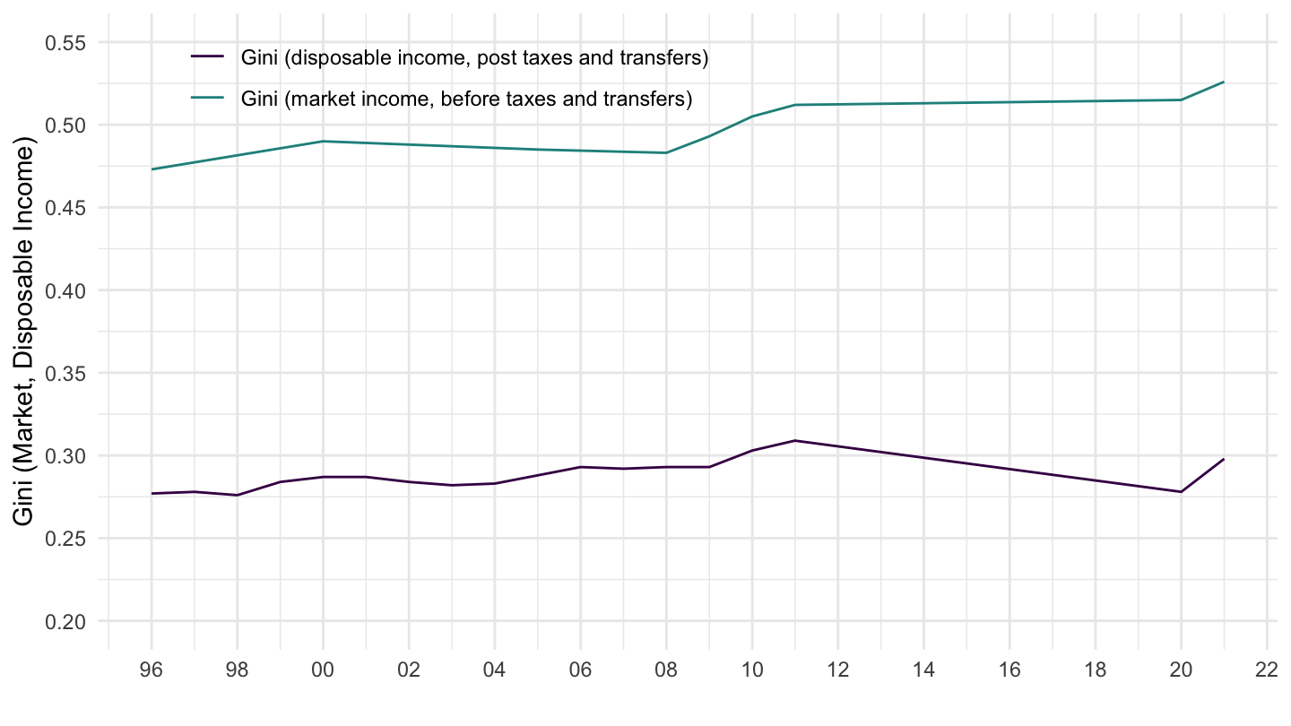
P90/P10 and S80/S20
(ref:P90P10-S80S20-FRA) Disposable Income Decile and Quintile Ratios
Code
IDD %>%
  filter(MEASURE %in% c("P90P10", "S80S20"),
         DEFINITION == "CURRENT",
         AGE == "TOT",
         LOCATION == "FRA") %>%
  year_to_date %>%
  left_join(IDD_var$MEASURE, by = "MEASURE") %>%
  ggplot() + ylab("P90/P10 and S80/S20") + xlab("") + theme_minimal() +
  geom_line(aes(x = date, y = obsValue, color = Measure)) +
  scale_color_manual(values = viridis(3)[1:2]) +
  scale_x_date(breaks = seq(1920, 2025, 2) %>% paste0("-01-01") %>% as.Date,
               labels = date_format("%y")) +
  scale_y_continuous(breaks = seq(0, 60, 0.1)) +
  theme(legend.position = c(0.3, 0.9),
        legend.title = element_blank())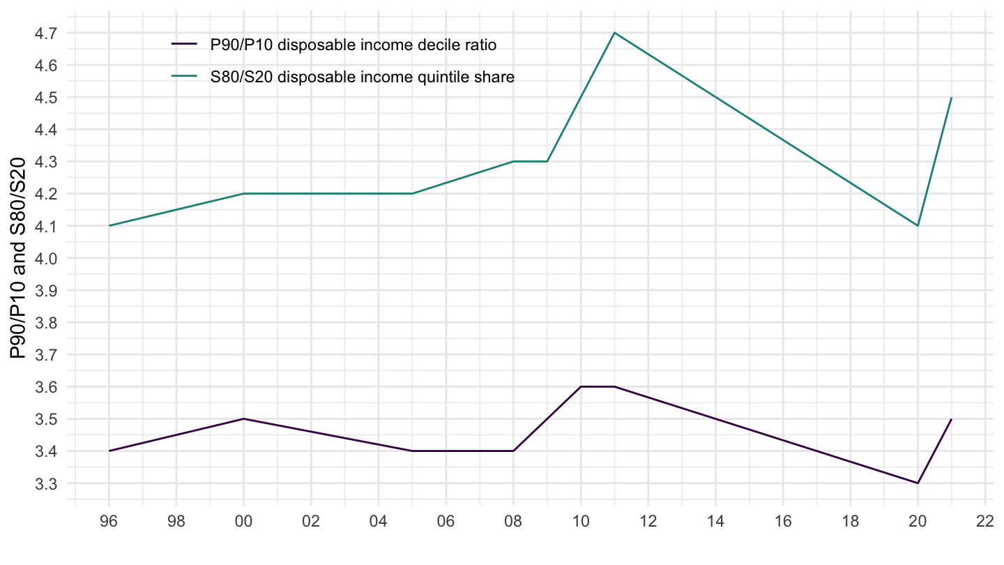
Germany
GINI and GINIB
(ref:GINI-GINIB-DEU) Gini Indicators in Germany: Market and Disposable Income
Code
IDD %>%
  filter(MEASURE %in% c("GINIB", "GINI"),
         DEFINITION == "CURRENT",
         AGE == "TOT",
         LOCATION == "DEU") %>%
  year_to_date %>%
  left_join(IDD_var$MEASURE, by = "MEASURE") %>%
  ggplot() + ylab("Gini (Market, Disposable Income)") + xlab("") + theme_minimal() +
  geom_line(aes(x = date, y = obsValue, color = Measure)) +
  scale_color_manual(values = viridis(3)[1:2]) +
  scale_x_date(breaks = seq(1920, 2025, 2) %>% paste0("-01-01") %>% as.Date,
               labels = date_format("%y")) +
  scale_y_continuous(breaks = 0.01*seq(0, 60, 5),
                     limits = c(0.2, 0.55)) +
  theme(legend.position = c(0.3, 0.9),
        legend.title = element_blank())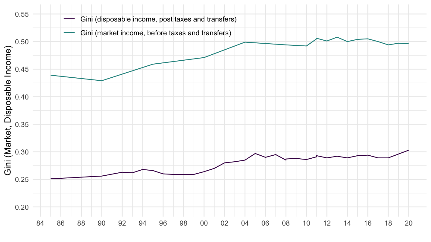
P90/P10 and S80/S20
(ref:P90P10-S80S20-DEU) Disposable Income Decile and Quintile Ratios
Code
IDD %>%
  filter(MEASURE %in% c("P90P10", "S80S20"),
         DEFINITION == "CURRENT",
         AGE == "TOT",
         LOCATION == "DEU",
         METHODO == "METH2012") %>%
  year_to_date %>%
  left_join(IDD_var$MEASURE, by = "MEASURE") %>%
  ggplot() + ylab("P90/P10 and S80/S20") + xlab("") + theme_minimal() +
  geom_line(aes(x = date, y = obsValue, color = Measure)) +
  scale_color_manual(values = viridis(3)[1:2]) +
  scale_x_date(breaks = seq(1920, 2025, 2) %>% paste0("-01-01") %>% as.Date,
               labels = date_format("%y")) +
  scale_y_continuous(breaks = seq(0, 60, 0.1)) +
  theme(legend.position = c(0.3, 0.9),
        legend.title = element_blank())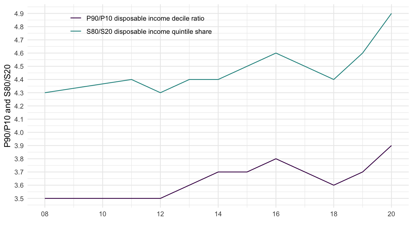
Gini
Table
Code
IDD %>%
  filter(MEASURE == "GINI",
         AGE == "TOT",
         obsTime %in% c("2018", "1998", "2008")) %>%
  left_join(IDD_var$LOCATION, by = "LOCATION") %>%
  select(-LOCATION) %>%
  select_if(~ n_distinct(.) > 1) %>%
  spread(obsTime, obsValue) %>%
  arrange(`2018`) %>%
  mutate(Flag = gsub(" ", "-", str_to_lower(gsub(" ", "-", Location))),
         Flag = paste0('<img src="../../icon/flag/vsmall/', Flag, '.png" alt="Flag">')) %>%
  select(Flag, everything()) %>%
  {if (is_html_output()) datatable(., filter = 'top', rownames = F, escape = F) else .}
France, Germany, United States
Code
IDD %>%
  filter(MEASURE == "GINI",
         AGE == "TOT",
         LOCATION %in% c("FRA", "DEU", "USA")) %>%
  year_to_date %>%
  left_join(IDD_var$LOCATION, by = c("LOCATION")) %>%
  left_join(colors, by = c("Location" = "country")) %>%
  ggplot() + geom_line(aes(x = date, y = obsValue, color = color)) +
  scale_color_identity() + theme_minimal() + add_3flags +
  scale_x_date(breaks = seq(1920, 2025, 2) %>% paste0("-01-01") %>% as.Date,
               labels = date_format("%y")) +
  theme(legend.position = c(0.25, 0.9),
        legend.title = element_blank()) +
  scale_y_continuous(breaks = 0.01*seq(0, 50, 2)) +
  ylab("Gini Index") + xlab("")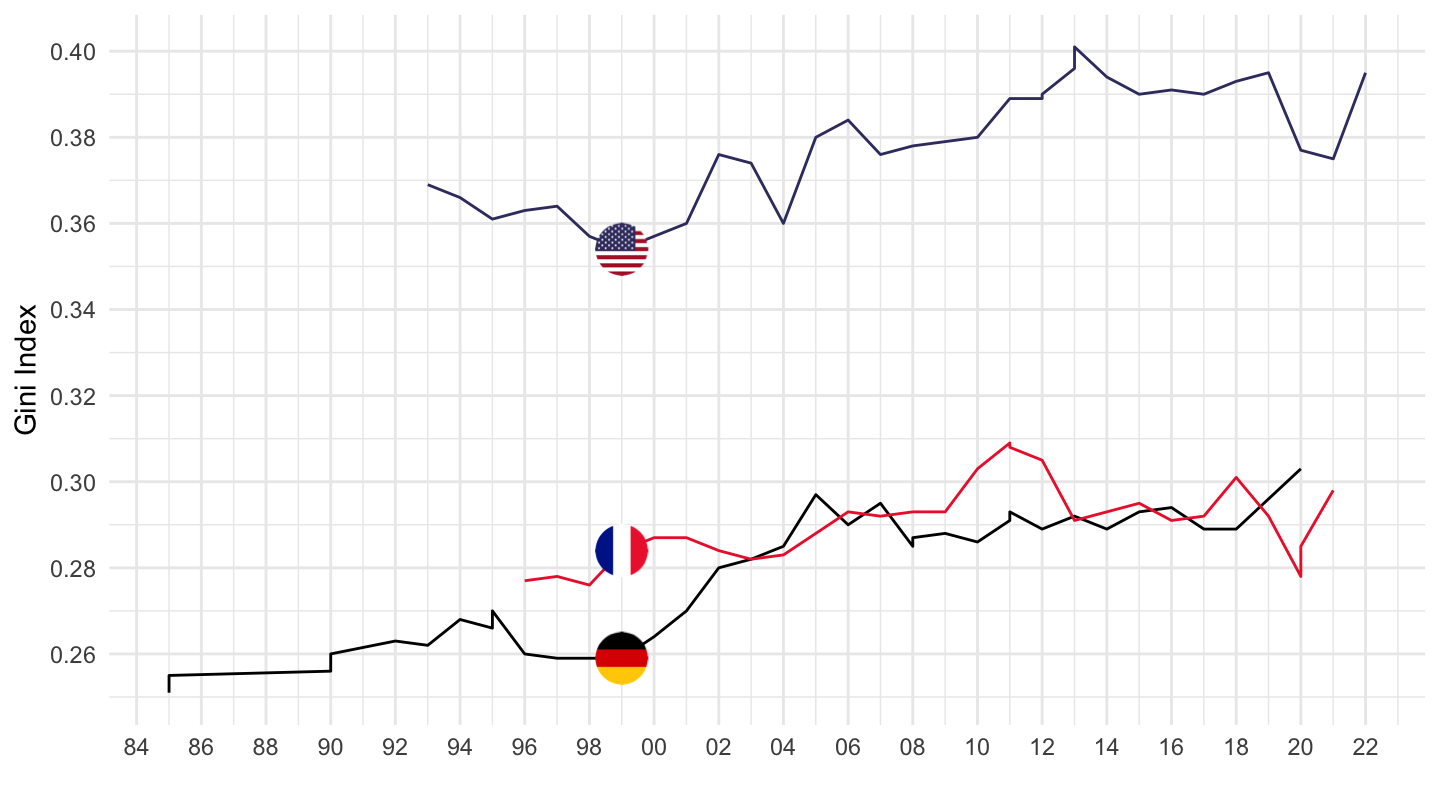
Inequality in Germany and France
All population
Code
IDD %>%
  filter(MEASURE == "GINI",
         AGE == "TOT",
         LOCATION %in% c("FRA", "DEU")) %>%
  year_to_date %>%
  left_join(IDD_var$LOCATION, by = c("LOCATION")) %>%
  left_join(colors, by = c("Location" = "country")) %>%
  ggplot() + geom_line(aes(x = date, y = obsValue, color = color)) +
  scale_color_identity() + theme_minimal() + add_2flags +
  scale_x_date(breaks = seq(1920, 2025, 2) %>% paste0("-01-01") %>% as.Date,
               labels = date_format("%y")) +
  theme(legend.position = c(0.25, 0.9),
        legend.title = element_blank()) +
  scale_y_continuous(breaks = 0.01*seq(0, 50, 2)) +
  ylab("Gini Index") + xlab("")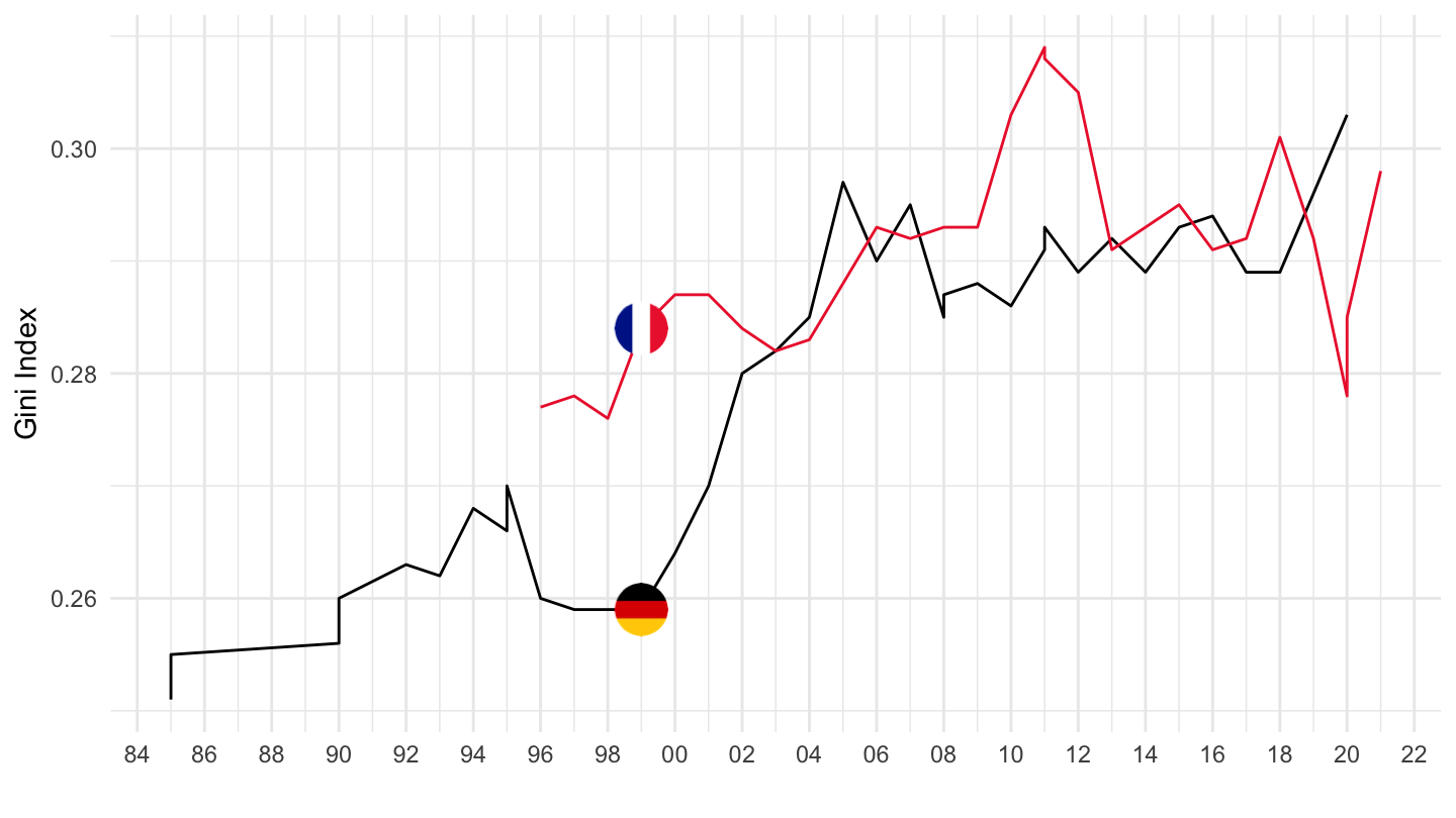
Age group 76+: mean disposable income (current prices)
Code
IDD %>%
  filter(MEASURE == "INCAC7",
         LOCATION %in% c("FRA", "DEU"),
         DEFINITION == "CURRENT") %>%
  year_to_date %>%
  left_join(IDD_var$LOCATION, by = c("LOCATION")) %>%
  left_join(colors, by = c("Location" = "country")) %>%
  ggplot() + geom_line(aes(x = date, y = obsValue, color = color)) +
  scale_color_identity() + theme_minimal() + add_2flags +
  scale_x_date(breaks = seq(1920, 2025, 2) %>% paste0("-01-01") %>% as.Date,
               labels = date_format("%y")) +
  theme(legend.position = c(0.25, 0.9),
        legend.title = element_blank()) +
  scale_y_continuous(breaks = seq(10000, 50000, 1000)) +
  ylab("Age group 76+: mean disposable income (current prices)") + xlab("")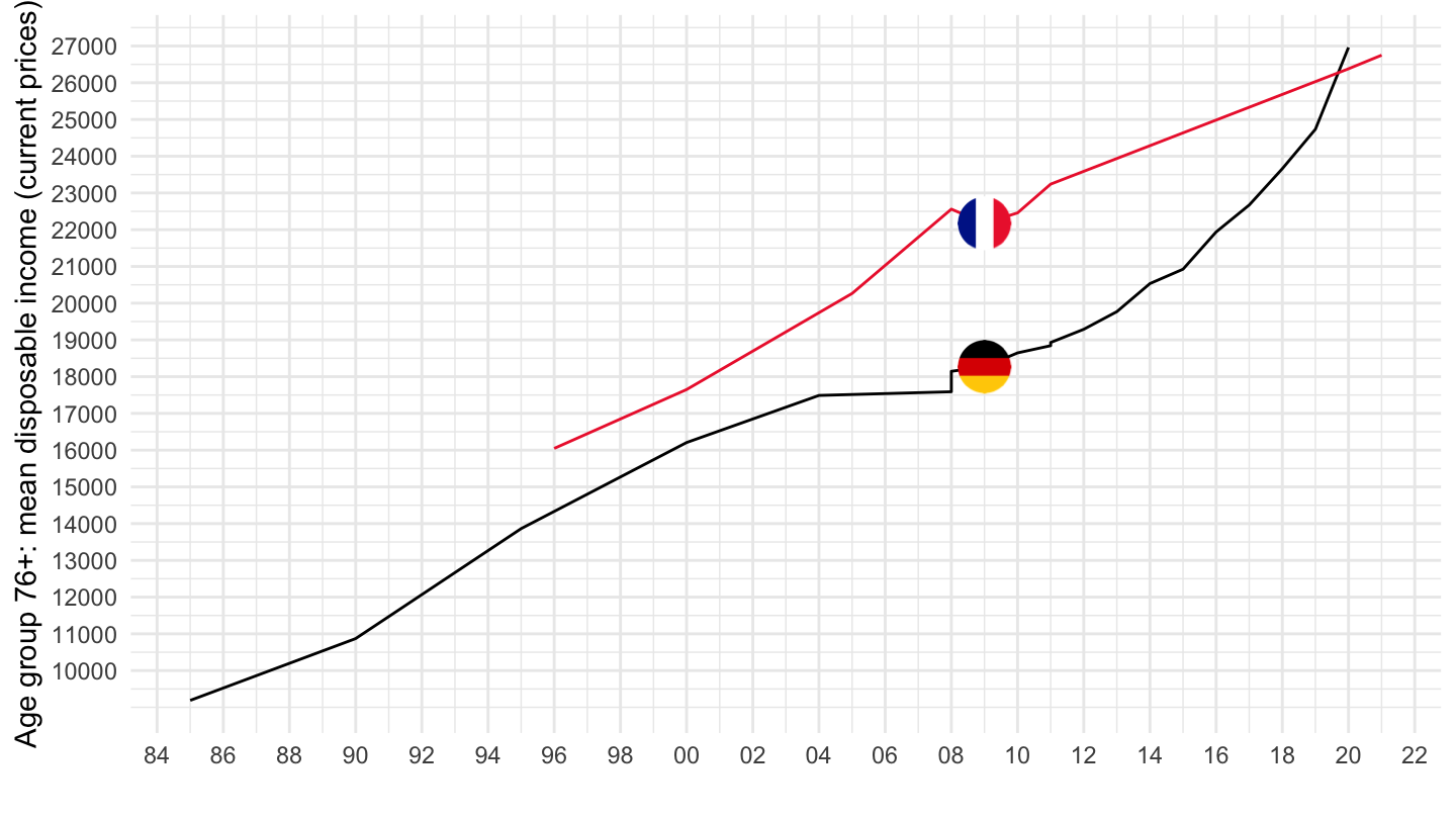
Age group 66-75: mean disposable income (current prices)
Code
IDD %>%
  filter(MEASURE == "INCAC6",
         LOCATION %in% c("FRA", "DEU"),
         DEFINITION == "CURRENT") %>%
  year_to_date %>%
  left_join(IDD_var$LOCATION, by = c("LOCATION")) %>%
  left_join(colors, by = c("Location" = "country")) %>%
  ggplot() + geom_line(aes(x = date, y = obsValue, color = color)) +
  scale_color_identity() + theme_minimal() + add_2flags +
  scale_x_date(breaks = seq(1920, 2025, 2) %>% paste0("-01-01") %>% as.Date,
               labels = date_format("%y")) +
  theme(legend.position = c(0.25, 0.9),
        legend.title = element_blank()) +
  scale_y_continuous(breaks = seq(10000, 50000, 1000)) +
  ylab("Age group 66-75: mean disposable income (current prices)") + xlab("")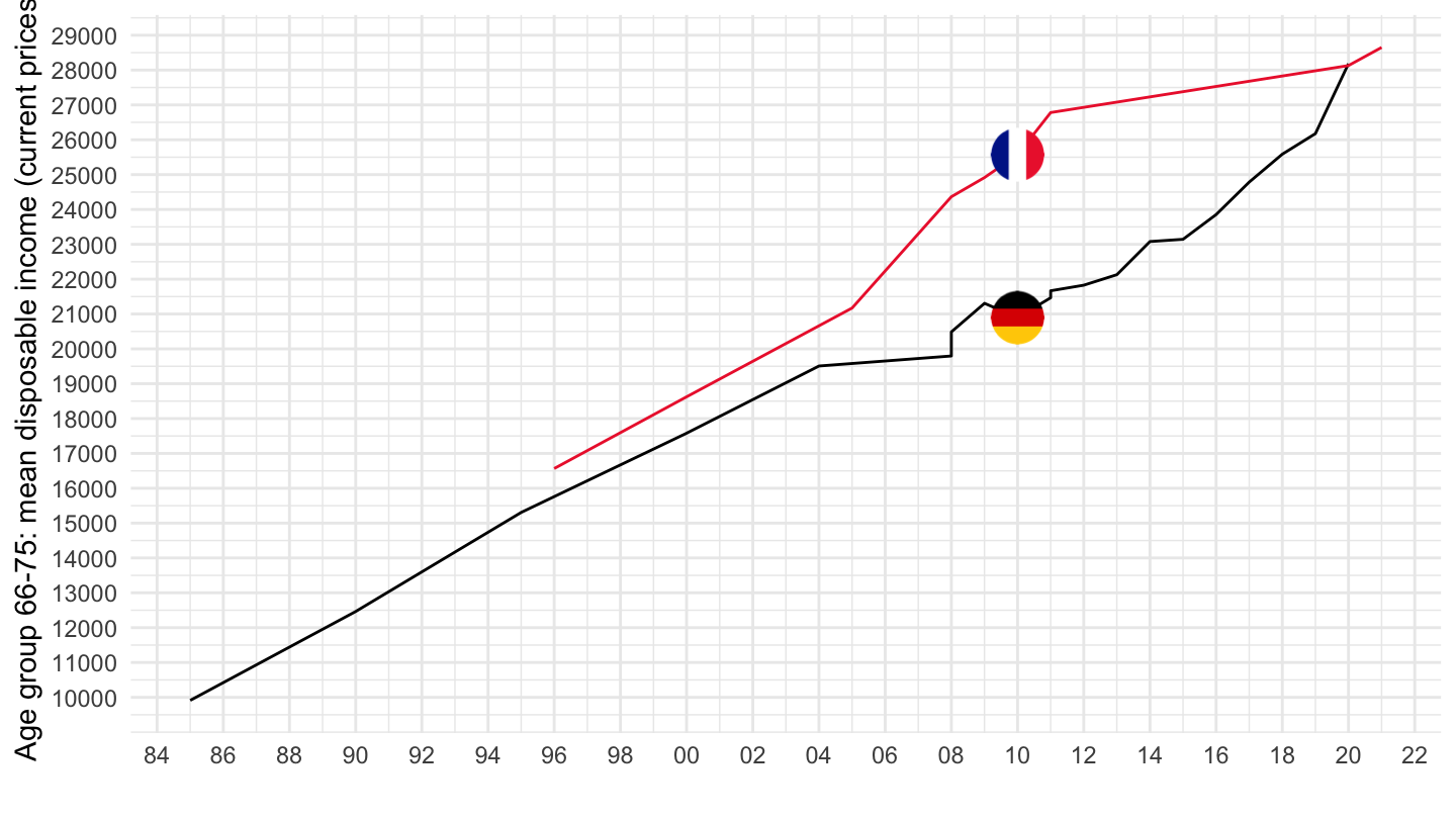
Age group 41-50: mean disposable income (current prices)
Code
IDD %>%
  filter(MEASURE == "INCAC4",
         LOCATION %in% c("FRA", "DEU"),
         DEFINITION == "CURRENT") %>%
  year_to_date %>%
  left_join(IDD_var$LOCATION, by = c("LOCATION")) %>%
  left_join(colors, by = c("Location" = "country")) %>%
  ggplot() + geom_line(aes(x = date, y = obsValue, color = color)) +
  scale_color_identity() + theme_minimal() + add_2flags +
  scale_x_date(breaks = seq(1920, 2025, 2) %>% paste0("-01-01") %>% as.Date,
               labels = date_format("%y")) +
  theme(legend.position = c(0.25, 0.9),
        legend.title = element_blank()) +
  scale_y_continuous(breaks = seq(10000, 50000, 1000)) +
  ylab("Age group 41-50: mean disposable income (current prices)") + xlab("")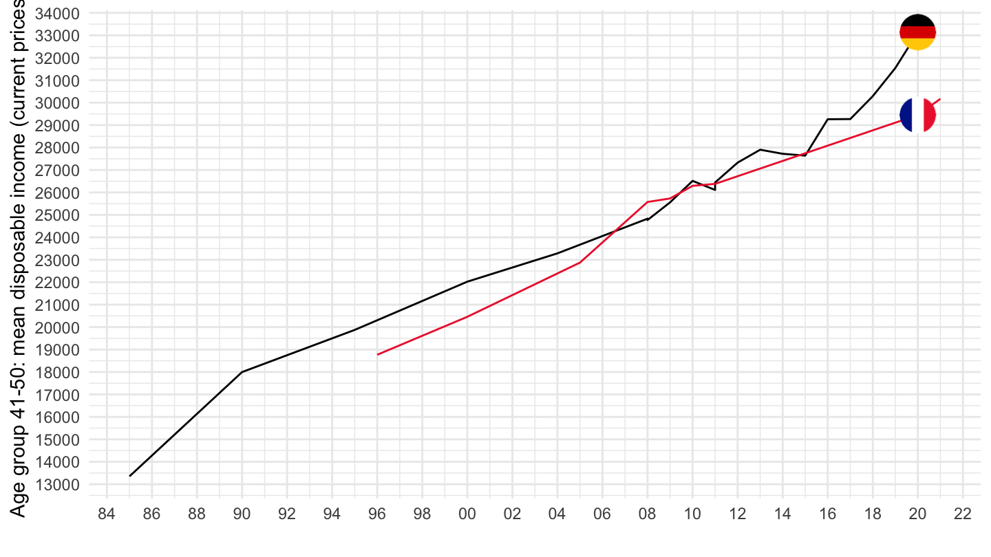
Age group 26-40: mean disposable income (current prices)
Code
# pdf(encoding = "ISOLatin9.enc")
IDD %>%
  filter(MEASURE == "INCAC3",
         LOCATION %in% c("FRA", "DEU"),
         DEFINITION == "CURRENT") %>%
  year_to_date %>%
  left_join(IDD_var$LOCATION, by = c("LOCATION")) %>%
  left_join(colors, by = c("Location" = "country")) %>%
  ggplot() + geom_line(aes(x = date, y = obsValue, color = color)) +
  scale_color_identity() + theme_minimal() + add_2flags +
  scale_x_date(breaks = seq(1920, 2025, 2) %>% paste0("-01-01") %>% as.Date,
               labels = date_format("%y")) +
  theme(legend.position = c(0.25, 0.9),
        legend.title = element_blank()) +
  scale_y_continuous(breaks = seq(10000, 50000, 1000),
                     labels = scales::dollar_format(accuracy = 1, suffix = "\u20ac", prefix = "")) +
  ylab("Age group 26-40: mean disposable income (current prices)") + xlab("")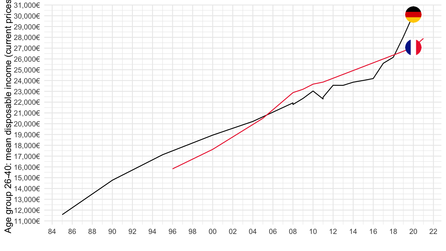
INCHCTOTAL
Code
IDD %>%
  filter(MEASURE == "INCHCTOTAL",
         LOCATION %in% c("FRA", "DEU"),
         DEFINITION == "CURRENT") %>%
  year_to_date %>%
  left_join(IDD_var$LOCATION, by = c("LOCATION")) %>%
  left_join(colors, by = c("Location" = "country")) %>%
  ggplot() + geom_line(aes(x = date, y = obsValue, color = color)) +
  scale_color_identity() + theme_minimal() + add_2flags +
  scale_x_date(breaks = seq(1920, 2025, 2) %>% paste0("-01-01") %>% as.Date,
               labels = date_format("%y")) +
  theme(legend.position = c(0.25, 0.9),
        legend.title = element_blank()) +
  scale_y_continuous(breaks = seq(10000, 50000, 1000),
                     labels = scales::dollar_format(accuracy = 1, suffix = "\u20ac", prefix = "")) +
  ylab("All working-age household types: mean disposable income") + xlab("")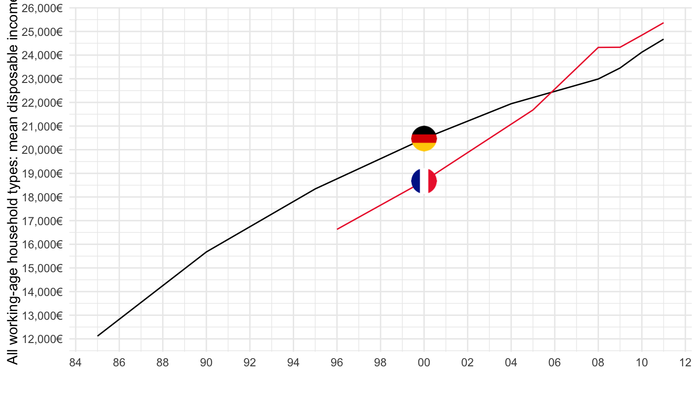
P90/P10 disposable income decile ratio
Code
IDD %>%
  filter(MEASURE == "P90P10",
         LOCATION %in% c("FRA", "DEU"),
         DEFINITION == "CURRENT",
         AGE == "TOT") %>%
  year_to_date %>%
  arrange(LOCATION, date) %>%
  filter(date >= as.Date("1994-01-01")) %>%
  left_join(IDD_var$LOCATION, by = c("LOCATION")) %>%
  left_join(colors, by = c("Location" = "country")) %>%
  ggplot() + geom_line(aes(x = date, y = obsValue, color = color)) +
  scale_color_identity() + theme_minimal() + add_2flags +
  scale_x_date(breaks = seq(1920, 2025, 2) %>% paste0("-01-01") %>% as.Date,
               labels = date_format("%y")) +
  theme(legend.position = c(0.25, 0.9),
        legend.title = element_blank()) +
  scale_y_continuous(breaks = seq(1, 5, 0.1)) +
  ylab("P90/P10 disposable income decile ratio") + xlab("")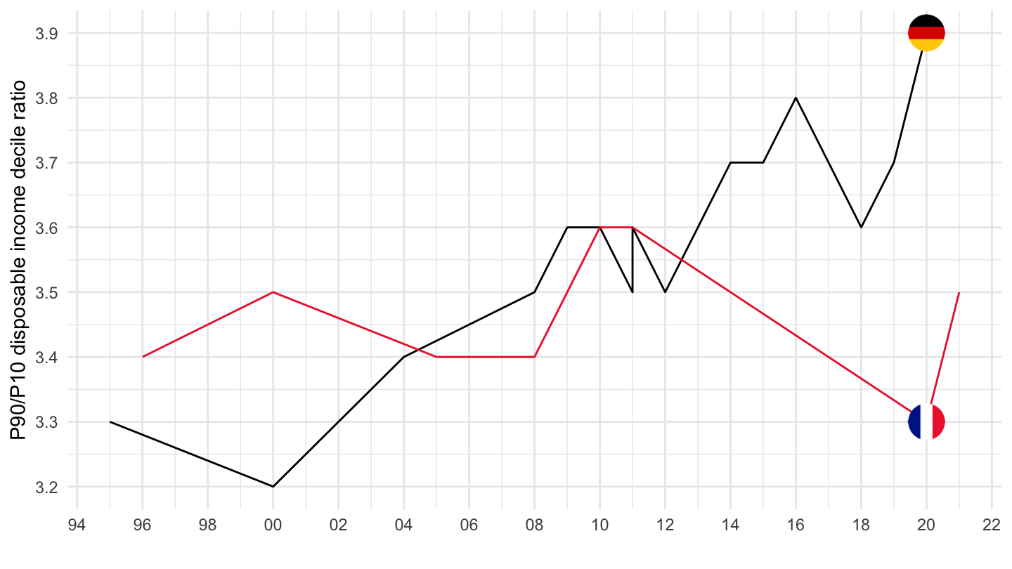
P50/P10 disposable income decile ratio
Code
IDD %>%
  filter(MEASURE == "P50P10",
         LOCATION %in% c("FRA", "DEU"),
         DEFINITION == "CURRENT",
         AGE == "TOT") %>%
  year_to_date %>%
  arrange(LOCATION, date) %>%
  left_join(IDD_var$LOCATION, by = c("LOCATION")) %>%
  left_join(colors, by = c("Location" = "country")) %>%
  ggplot() + geom_line(aes(x = date, y = obsValue, color = color)) +
  scale_color_identity() + theme_minimal() + add_2flags +
  scale_x_date(breaks = seq(1920, 2025, 2) %>% paste0("-01-01") %>% as.Date,
               labels = date_format("%y")) +
  theme(legend.position = c(0.25, 0.9),
        legend.title = element_blank()) +
  scale_y_continuous(breaks = seq(1, 5, 0.1)) +
  ylab("P90/P10 disposable income decile ratio") + xlab("")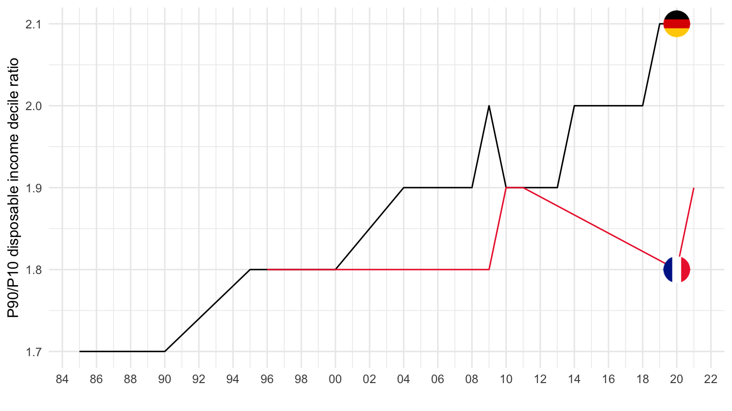
S80/S20 disposable income quintile ratio
Code
IDD %>%
  filter(MEASURE == "S80S20",
         LOCATION %in% c("FRA", "DEU"),
         DEFINITION == "CURRENT",
         AGE == "TOT") %>%
  year_to_date %>%
  arrange(LOCATION, date) %>%
  left_join(IDD_var$LOCATION, by = c("LOCATION")) %>%
  left_join(colors, by = c("Location" = "country")) %>%
  ggplot() + geom_line(aes(x = date, y = obsValue, color = color)) +
  scale_color_identity() + theme_minimal() + add_2flags +
  scale_x_date(breaks = seq(1920, 2025, 2) %>% paste0("-01-01") %>% as.Date,
               labels = date_format("%y")) +
  theme(legend.position = c(0.25, 0.9),
        legend.title = element_blank()) +
  scale_y_continuous(breaks = seq(1, 5, 0.1)) +
  ylab("S80/S20 disposable income quintile share") + xlab("")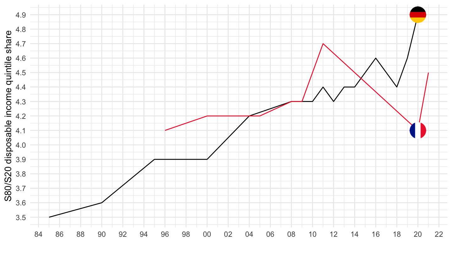
Poverty (France, Germany)
PVT5A
Code
IDD %>%
  filter(MEASURE == "PVT5A",
         DEFINITION == "CURRENT",
         AGE == "TOT",
         LOCATION %in% c("DEU", "FRA")) %>%
  year_to_date %>%
  left_join(IDD_var$LOCATION, by = c("LOCATION")) %>%
  left_join(colors, by = c("Location" = "country")) %>%
  ggplot() + geom_line(aes(x = date, y = obsValue, color = color)) +
  scale_color_identity() + theme_minimal() + add_2flags +
  scale_x_date(breaks = seq(1920, 2025, 2) %>% paste0("-01-01") %>% as.Date,
               labels = date_format("%y")) +
  scale_y_continuous(breaks = 0.01*seq(-7, 50, 1),
                     labels = percent_format(accuracy = 1)) +
  ylab("Poverty rate after taxes and transfers, Poverty line 50%") + xlab("")
PVT5B
Code
IDD %>%
  filter(MEASURE == "PVT5B",
         DEFINITION == "CURRENT",
         AGE == "TOT",
         LOCATION %in% c("DEU", "FRA")) %>%
  year_to_date %>%
  left_join(IDD_var$LOCATION, by = c("LOCATION")) %>%
  left_join(colors, by = c("Location" = "country")) %>%
  ggplot() + geom_line(aes(x = date, y = obsValue, color = color)) +
  scale_color_identity() + theme_minimal() + add_2flags +
  scale_x_date(breaks = seq(1920, 2025, 2) %>% paste0("-01-01") %>% as.Date,
               labels = date_format("%y")) +
  theme(legend.position = c(0.25, 0.9),
        legend.title = element_blank()) +
  scale_y_continuous(breaks = 0.01*seq(-7, 50, 1),
                     labels = percent_format(accuracy = 1)) +
  ylab("Poverty rate before taxes and transfers, Poverty line 50%") + xlab("")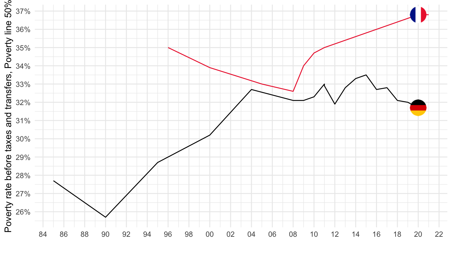
PALMA
Code
IDD %>%
  filter(MEASURE == "PALMA",
         DEFINITION == "CURRENT",
         AGE == "TOT",
         LOCATION %in% c("DEU", "FRA")) %>%
  year_to_date %>%
  left_join(IDD_var$LOCATION, by = c("LOCATION")) %>%
  left_join(colors, by = c("Location" = "country")) %>%
  ggplot() + geom_line(aes(x = date, y = obsValue, color = color)) +
  scale_color_identity() + theme_minimal() + add_2flags +
  scale_x_date(breaks = seq(1920, 2025, 2) %>% paste0("-01-01") %>% as.Date,
               labels = date_format("%y")) +
  theme(legend.position = c(0.25, 0.9),
        legend.title = element_blank()) +
  scale_y_continuous(breaks = seq(-7, 50, 0.05)) +
  ylab("Palma Ratio") + xlab("")
PVTAATOTAL
Code
IDD %>%
  filter(MEASURE == "PVTAATOTAL",
         DEFINITION == "CURRENT",
         AGE == "TOT",
         LOCATION %in% c("DEU", "FRA")) %>%
  year_to_date %>%
  left_join(IDD_var$LOCATION, by = c("LOCATION")) %>%
  left_join(colors, by = c("Location" = "country")) %>%
  ggplot() + geom_line(aes(x = date, y = obsValue, color = color)) +
  scale_color_identity() + theme_minimal() + add_2flags +
  scale_x_date(breaks = seq(1920, 2025, 2) %>% paste0("-01-01") %>% as.Date,
               labels = date_format("%y")) +
  theme(legend.position = c(0.25, 0.9),
        legend.title = element_blank()) +
  scale_y_continuous(breaks = 0.01*seq(-7, 50, 1),
                     labels = percent_format(accuracy = 1)) +
  ylab("Poverty Rate") + xlab("")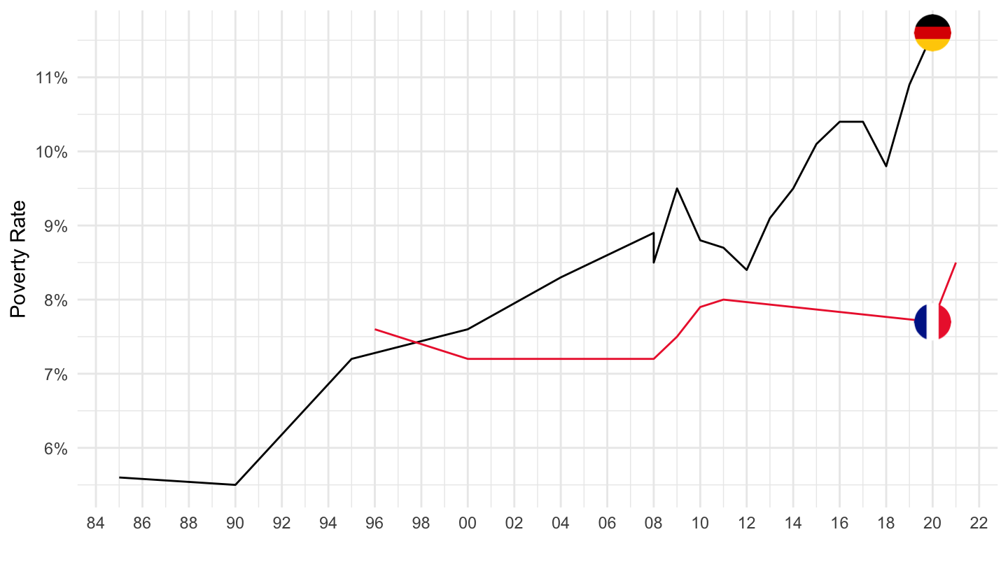
GINIB
Code
IDD %>%
  filter(MEASURE == "GINIB",
         DEFINITION == "CURRENT",
         AGE == "TOT",
         LOCATION %in% c("DEU", "FRA")) %>%
  year_to_date %>%
  left_join(IDD_var$LOCATION, by = c("LOCATION")) %>%
  left_join(colors, by = c("Location" = "country")) %>%
  ggplot() + geom_line(aes(x = date, y = obsValue, color = color)) +
  scale_color_identity() + theme_minimal() + add_2flags +
  scale_x_date(breaks = seq(1920, 2025, 2) %>% paste0("-01-01") %>% as.Date,
               labels = date_format("%y")) +
  theme(legend.position = c(0.25, 0.9),
        legend.title = element_blank()) +
  scale_y_continuous(breaks = 0.01*seq(-7, 60, 1),
                     labels = percent_format(accuracy = 1)) +
  ylab("Gini (Market Income)") + xlab("")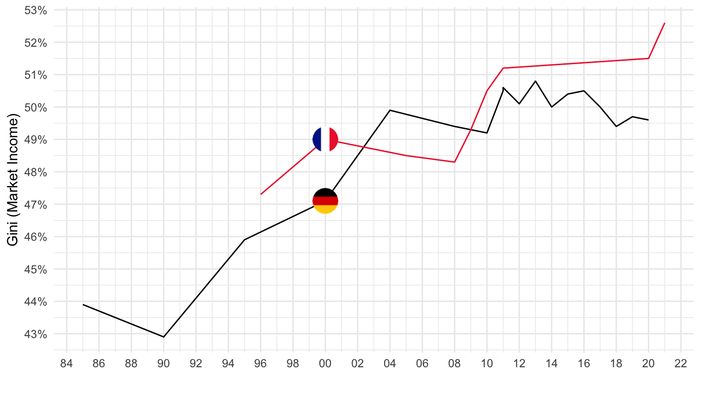
Poverty rate after taxes and transfers
Code
IDD %>%
  filter(MEASURE == "PVT5A",
         DEFINITION == "CURRENT",
         AGE == "TOT",
         LOCATION %in% c("DEU", "FRA")) %>%
  year_to_date %>%
  left_join(IDD_var$LOCATION, by = c("LOCATION")) %>%
  left_join(colors, by = c("Location" = "country")) %>%
  ggplot() + geom_line(aes(x = date, y = obsValue, color = color)) +
  scale_color_identity() + theme_minimal() + add_2flags +
  scale_x_date(breaks = seq(1920, 2025, 2) %>% paste0("-01-01") %>% as.Date,
               labels = date_format("%y")) +
  theme(legend.position = c(0.25, 0.9),
        legend.title = element_blank()) +
  scale_y_continuous(breaks = 0.01*seq(-7, 50, 1),
                     labels = percent_format(accuracy = 1)) +
  ylab("Poverty rate after taxes and transfers, Poverty line 50%") + xlab("")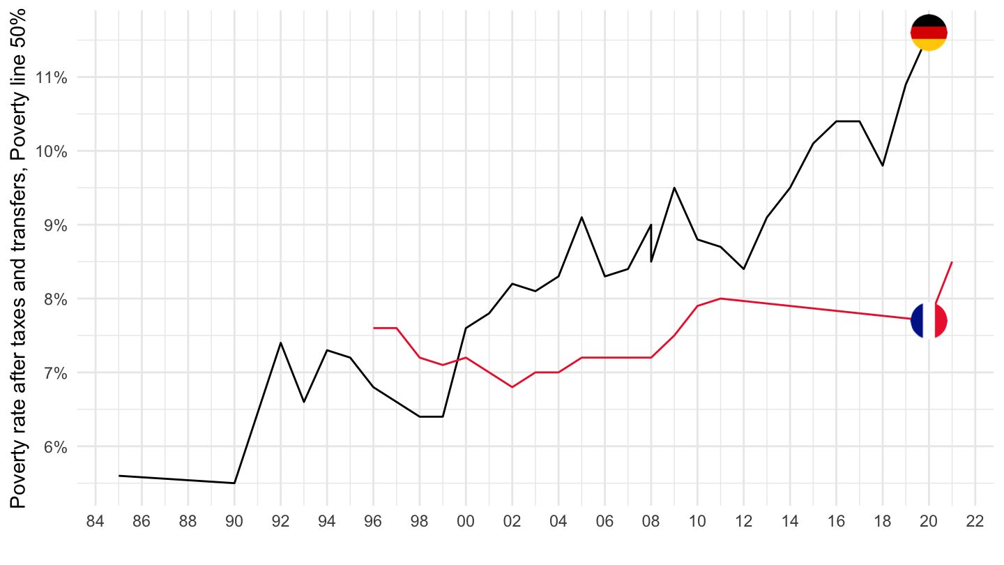
Poverty rate before taxes and transfers
Code
IDD %>%
  filter(MEASURE == "PVT5B",
         DEFINITION == "CURRENT",
         AGE == "TOT",
         LOCATION %in% c("DEU", "FRA")) %>%
  year_to_date %>%
  left_join(IDD_var$LOCATION, by = c("LOCATION")) %>%
  left_join(colors, by = c("Location" = "country")) %>%
  ggplot() + geom_line(aes(x = date, y = obsValue, color = color)) +
  scale_color_identity() + theme_minimal() + add_2flags +
  scale_x_date(breaks = seq(1920, 2025, 2) %>% paste0("-01-01") %>% as.Date,
               labels = date_format("%y")) +
  theme(legend.position = c(0.25, 0.9),
        legend.title = element_blank()) +
  scale_y_continuous(breaks = 0.01*seq(-7, 50, 1),
                     labels = percent_format(accuracy = 1)) +
  ylab("Poverty rate before taxes and transfers, Poverty line 50%") + xlab("")
Palma
Code
IDD %>%
  filter(MEASURE == "PALMA",
         DEFINITION == "CURRENT",
         AGE == "TOT",
         LOCATION %in% c("DEU", "FRA")) %>%
  year_to_date %>%
  left_join(IDD_var$LOCATION, by = c("LOCATION")) %>%
  left_join(colors, by = c("Location" = "country")) %>%
  ggplot() + geom_line(aes(x = date, y = obsValue, color = color)) +
  scale_color_identity() + theme_minimal() + add_2flags +
  scale_x_date(breaks = seq(1920, 2025, 2) %>% paste0("-01-01") %>% as.Date,
               labels = date_format("%y")) +
  theme(legend.position = c(0.25, 0.9),
        legend.title = element_blank()) +
  scale_y_continuous(breaks = seq(-7, 50, 0.05)) +
  ylab("Palma Ratio") + xlab("")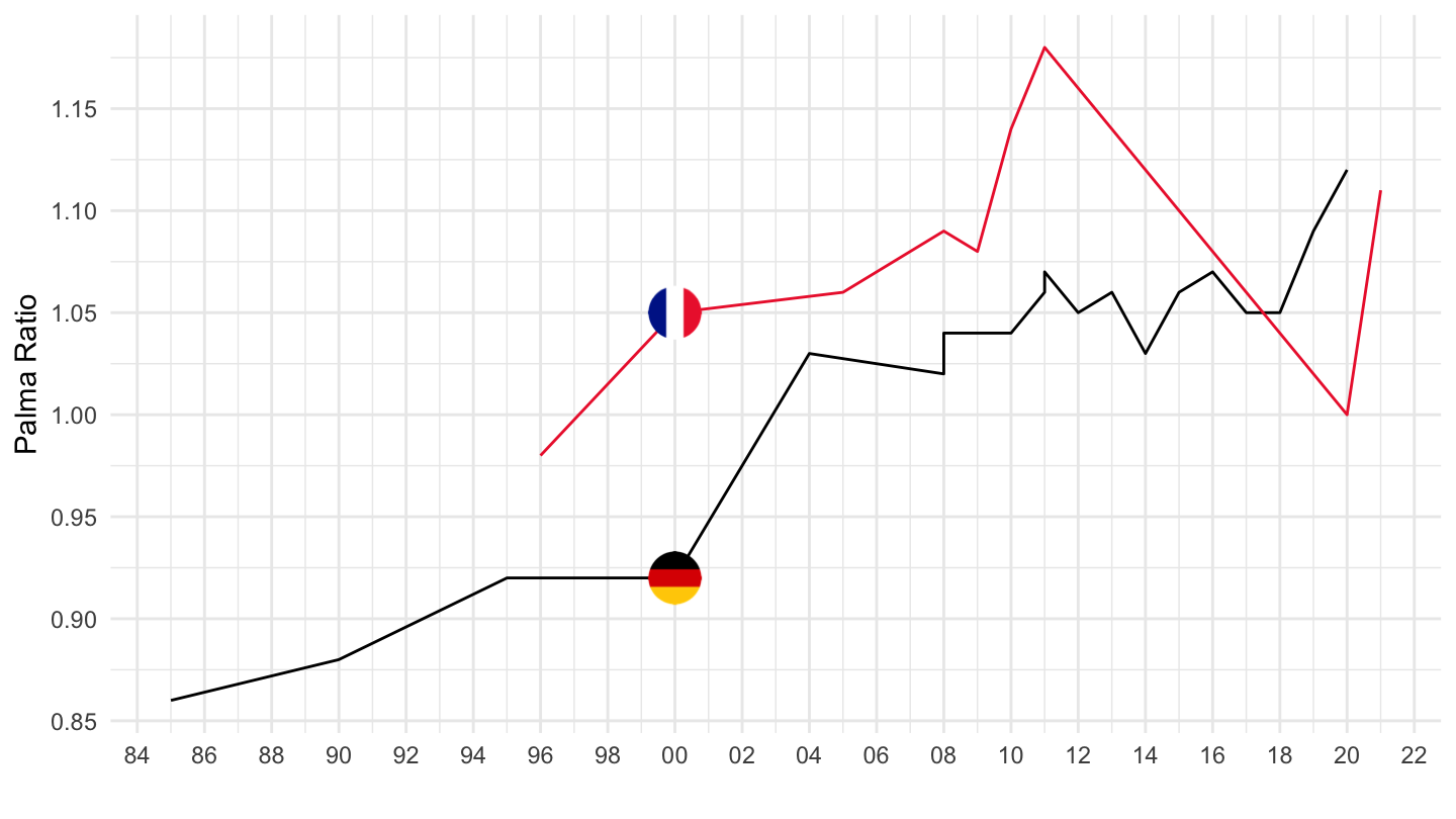
Poverty Rate
Code
IDD %>%
  filter(MEASURE == "PVTAATOTAL",
         DEFINITION == "CURRENT",
         AGE == "TOT",
         LOCATION %in% c("DEU", "FRA")) %>%
  year_to_date %>%
  left_join(IDD_var$LOCATION, by = c("LOCATION")) %>%
  left_join(colors, by = c("Location" = "country")) %>%
  ggplot() + geom_line(aes(x = date, y = obsValue, color = color)) +
  scale_color_identity() + theme_minimal() + add_2flags +
  scale_x_date(breaks = seq(1920, 2025, 2) %>% paste0("-01-01") %>% as.Date,
               labels = date_format("%y")) +
  theme(legend.position = c(0.25, 0.9),
        legend.title = element_blank()) +
  scale_y_continuous(breaks = 0.01*seq(-7, 50, 1),
                     labels = percent_format(accuracy = 1)) +
  ylab("Poverty Rate") + xlab("")
Gini
Code
IDD %>%
  filter(MEASURE == "GINI",
         AGE == "TOT",
         LOCATION %in% c("FRA", "DEU", "USA")) %>%
  year_to_date %>%
  left_join(IDD_var$LOCATION, by = c("LOCATION")) %>%
  left_join(colors, by = c("Location" = "country")) %>%
  ggplot() + geom_line(aes(x = date, y = obsValue, color = color)) +
  scale_color_identity() + theme_minimal() + add_3flags +
  scale_x_date(breaks = seq(1920, 2025, 2) %>% paste0("-01-01") %>% as.Date,
               labels = date_format("%y")) +
  theme(legend.position = c(0.25, 0.9),
        legend.title = element_blank()) +
  scale_y_continuous(breaks = 0.01*seq(0, 50, 2)) +
  ylab("Gini Index") + xlab("")