Balance of payments

Data - OECD

Info

Last observation: Quarterly: 2026-Q2 (N = 394) · Monthly: 2026-06 (N = 56) · Annual: 2025 (N = 5,009)

Last update of .parquet: 14 aoû 2026, 23:17. Last compile: 14 aoû 2026, 23:43

Structure

REF_AREA

COUNTERPART_AREA

MEASURE

ACCOUNTING_ENTRY

FS_ENTRY

FREQ

UNIT_MEASURE

ADJUSTMENT

OBS_STATUS

UNIT_MULT

CURRENCY

DECIMALS

Financial account

EU vs. US vs. DE vs. FR

All

BOP |>
  filter(MEASURE == "FA",
         REF_AREA %in% c("USA", "EU27_2020", "DEU", "FRA"),
         FREQ == "Q",
         UNIT_MEASURE == "USD_EXC",
         ACCOUNTING_ENTRY == "N") |>
  arrange(desc(obsTime)) |>
  quarter_to_date() |>
  
  arrange(desc(date)) |>
  mutate(Ref_area = ifelse(REF_AREA == "EU27_2020", "Europe", Ref_area)) |>
  left_join(colors, by = c("Ref_area" = "country")) |>
  mutate(color = ifelse(REF_AREA == "USA", color2, color)) |>
  mutate(obsValue = obsValue/100) |>
  #filter(date >= as.Date("1999-01-01")) %>%
  #filter(date <= as.Date("2021-01-01")) %>%
  ggplot() + geom_line(aes(x = date, y = obsValue, color = color)) + 
  theme_minimal() + xlab("") + ylab("Financial Account") +
  scale_color_identity() + add_4flags +
  scale_x_date(breaks = c(seq(1949, 2100, 5)) |> paste0("-01-01") |> as.Date(),
               labels = date_format("%Y")) +
  scale_y_continuous(breaks = seq(-10000, 10000, 500)) +
  geom_hline(yintercept = 0, linetype = "dashed", color = "black")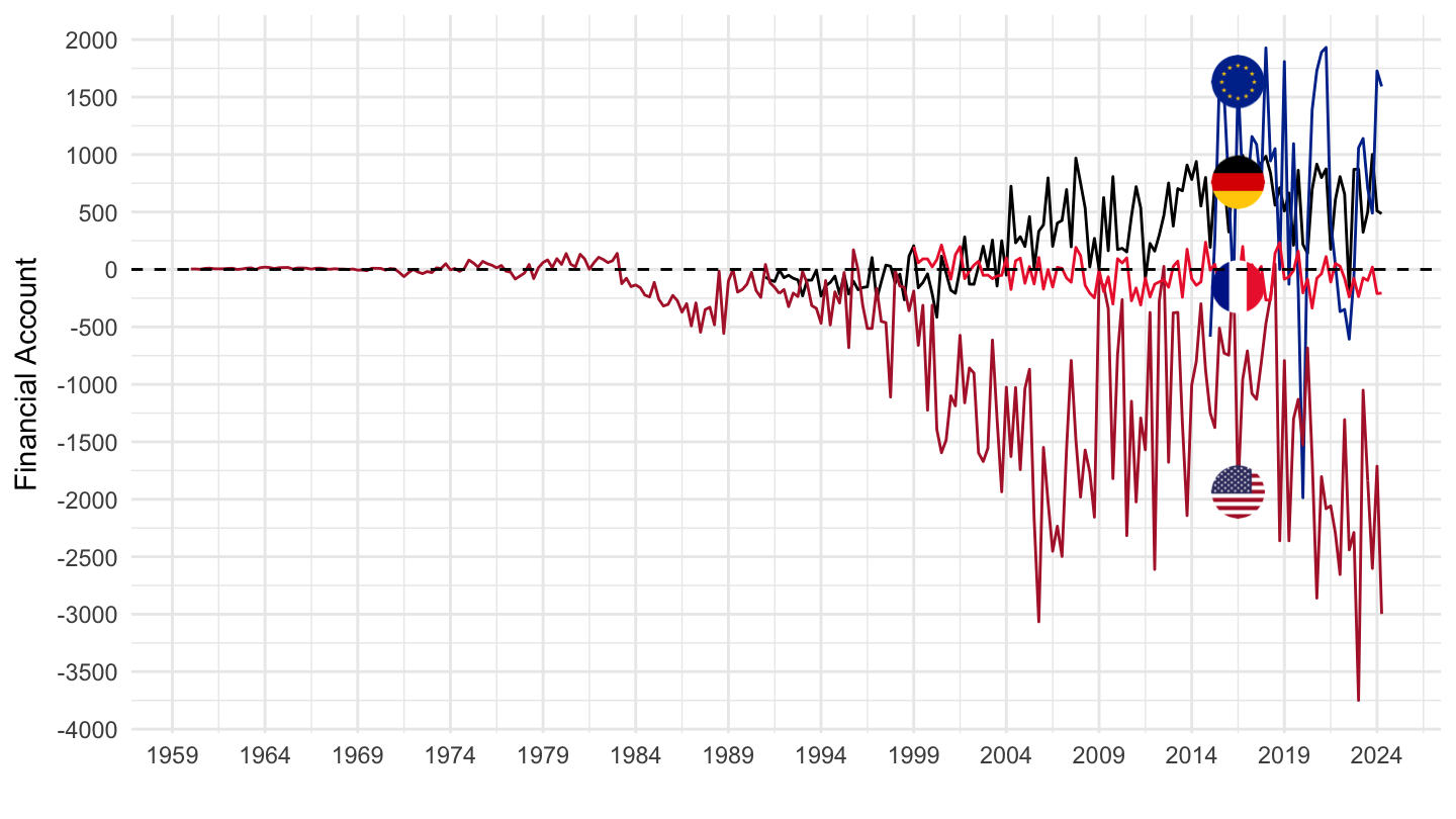

1999-

BOP |>
  filter(MEASURE == "FA",
         REF_AREA %in% c("USA", "EU27_2020", "DEU", "FRA"),
         FREQ == "Q",
         UNIT_MEASURE == "USD_EXC",
         ACCOUNTING_ENTRY == "N") |>
  quarter_to_date() |>
  
  arrange(desc(date)) |>
  mutate(Ref_area = ifelse(REF_AREA == "EU27_2020", "Europe", Ref_area)) |>
  left_join(colors, by = c("Ref_area" = "country")) |>
  mutate(color = ifelse(REF_AREA == "USA", color2, color)) |>
  mutate(obsValue = obsValue/100) |>
  filter(date >= as.Date("1999-01-01")) |>
  
  #filter(date <= as.Date("2021-01-01")) %>%
  ggplot() + geom_line(aes(x = date, y = obsValue, color = color)) + 
  theme_minimal() + xlab("") + ylab("Financial Account") +
  scale_color_identity() + add_4flags +
  scale_x_date(breaks = c(seq(1999, 2100, 5)) |> paste0("-01-01") |> as.Date(),
               labels = date_format("%Y")) +
  scale_y_continuous(breaks = seq(-10000, 10000, 500)) +
  geom_hline(yintercept = 0, linetype = "dashed", color = "black")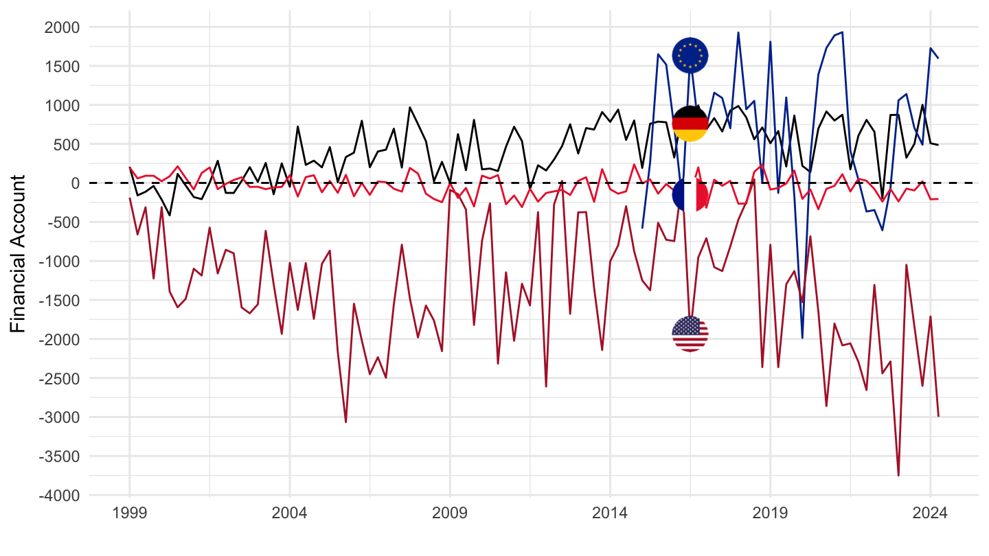

Current account (CA, % of GDP)

Greece, EU, US, France

1999-

Quarterly

BOP |>
  filter(MEASURE == "CA",
         REF_AREA %in% c("FRA", "GRC", "USA", "EU27_2020"),
         FREQ == "Q",
         UNIT_MEASURE == "PT_B1GQ") |>
  quarter_to_date() |>
  
  arrange(desc(date)) |>
  mutate(Ref_area = ifelse(REF_AREA == "EU27_2020", "Europe", Ref_area)) |>
  left_join(colors, by = c("Ref_area" = "country")) |>
  mutate(color = ifelse(REF_AREA == "USA", color2, color)) |>
  mutate(obsValue = obsValue/100) |>
  filter(date >= as.Date("1999-01-01")) |>
  
  #filter(date <= as.Date("2021-01-01")) %>%
  ggplot() + geom_line(aes(x = date, y = obsValue, color = color)) + 
  theme_minimal() + xlab("") + ylab("Current Account, % of GDP") +
  scale_color_identity() + add_2flags +
  scale_x_date(breaks = c(seq(1990, 2100, 2)) |> paste0("-01-01") |> as.Date(),
               labels = date_format("%Y")) +
  scale_y_continuous(breaks = 0.01*seq(-60, 60, 1),
                     labels = scales::percent_format(accuracy = 1)) +
  geom_hline(yintercept = 0, linetype = "dashed", color = "black") +
  geom_label(data = . %>% filter(date == max(date)),
             aes(x = date, y = obsValue, label = percent(obsValue), color = color))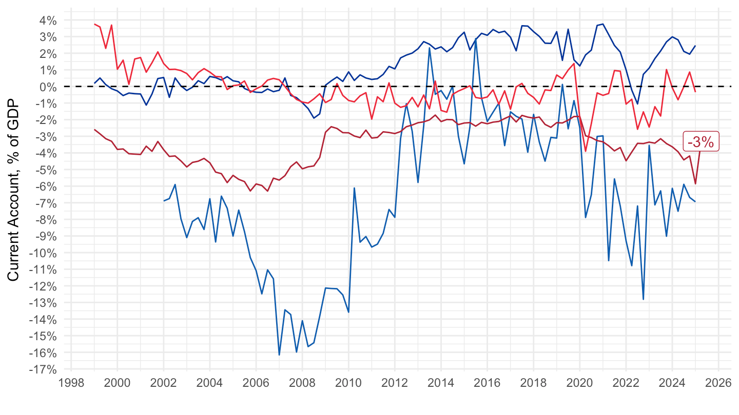

Smoothed

BOP |>
  filter(MEASURE == "CA",
         REF_AREA %in% c("FRA", "GRC", "USA", "EU27_2020"),
         FREQ == "Q",
         UNIT_MEASURE == "PT_B1GQ") |>
  quarter_to_date() |>
  
  arrange(desc(date)) |>
  mutate(Ref_area = ifelse(REF_AREA == "EU27_2020", "Europe", Ref_area)) |>
  left_join(colors, by = c("Ref_area" = "country")) |>
  mutate(color = ifelse(REF_AREA == "USA", color2, color)) |>
  mutate(obsValue = obsValue/100) |>
  group_by(REF_AREA) |>
  arrange(date) |>
  mutate(obsValue = zoo::rollmean(obsValue, k = 4, fill = NA, align = "right")) |>
  ungroup() |>
  filter(date >= as.Date("1999-01-01")) |>
  
  #filter(date <= as.Date("2021-01-01")) %>%
  ggplot() + geom_line(aes(x = date, y = obsValue, color = color)) + 
  theme_minimal() + xlab("") + ylab("Current Account, % of GDP") +
  scale_color_identity() + add_4flags +
  scale_x_date(breaks = c(seq(1990, 2100, 2)) |> paste0("-01-01") |> as.Date(),
               labels = date_format("%Y")) +
  scale_y_continuous(breaks = 0.01*seq(-60, 60, 1),
                     labels = scales::percent_format(accuracy = 1)) +
  geom_hline(yintercept = 0, linetype = "dashed", color = "black") +
  geom_label(data = . %>% filter(date == max(date)),
             aes(x = date, y = obsValue, label = percent(obsValue), color = color))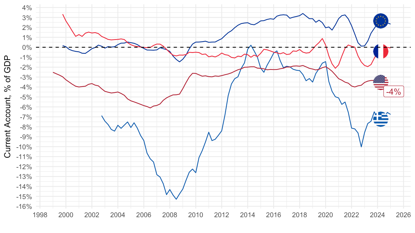

Smoothed

BOP |>
  filter(MEASURE == "CA",
         REF_AREA %in% c("FRA", "GRC", "PRT", "IRL"),
         FREQ == "Q",
         UNIT_MEASURE == "PT_B1GQ") |>
  quarter_to_date() |>
  filter(date <= as.Date("2017-01-01")) |>
  
  arrange(desc(date)) |>
  mutate(Ref_area = ifelse(REF_AREA == "EU27_2020", "Europe", Ref_area)) |>
  left_join(colors, by = c("Ref_area" = "country")) |>
  mutate(color = ifelse(REF_AREA == "USA", color2, color)) |>
  mutate(obsValue = obsValue/100) |>
  group_by(REF_AREA) |>
  arrange(date) |>
  mutate(obsValue = zoo::rollmean(obsValue, k = 4, fill = NA, align = "right")) |>
  ungroup() |>
  filter(date >= as.Date("1999-01-01")) |>
  
  #filter(date <= as.Date("2021-01-01")) %>%
  ggplot() + geom_line(aes(x = date, y = obsValue, color = color)) + 
  theme_minimal() + xlab("") + ylab("Current Account, % of GDP") +
  scale_color_identity() + add_4flags +
  scale_x_date(breaks = c(seq(1990, 2100, 2)) |> paste0("-01-01") |> as.Date(),
               labels = date_format("%Y")) +
  scale_y_continuous(breaks = 0.01*seq(-60, 60, 1),
                     labels = scales::percent_format(accuracy = 1)) +
  geom_hline(yintercept = 0, linetype = "dashed", color = "black") +
  geom_label(data = . %>% filter(date == max(date)),
             aes(x = date, y = obsValue, label = percent(obsValue), color = color))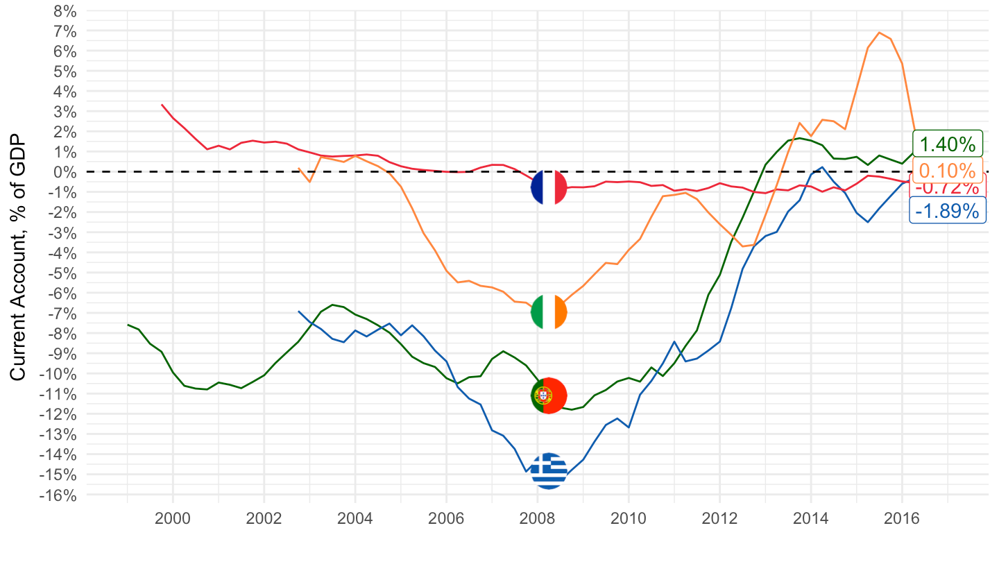

2003-

Smoothed

BOP |>
  filter(MEASURE == "CA",
         REF_AREA %in% c("FRA", "GRC", "USA", "EU27_2020", "ITA"),
         FREQ == "Q",
         UNIT_MEASURE == "PT_B1GQ") |>
  quarter_to_date() |>
  
  arrange(desc(date)) |>
  mutate(Ref_area = ifelse(REF_AREA == "EU27_2020", "Europe", Ref_area)) |>
  left_join(colors, by = c("Ref_area" = "country")) |>
  mutate(color = ifelse(REF_AREA == "USA", color2, color)) |>
  mutate(obsValue = obsValue/100) |>
  group_by(REF_AREA) |>
  arrange(date) |>
  mutate(obsValue = zoo::rollmean(obsValue, k = 4, fill = NA, align = "right")) |>
  ungroup() |>
  filter(date >= as.Date("2003-01-01")) |>
  
  #filter(date <= as.Date("2021-01-01")) %>%
  ggplot() + geom_line(aes(x = date, y = obsValue, color = color)) + 
  theme_minimal() + xlab("") + ylab("Current Account, % of GDP") +
  scale_color_identity() + add_5flags +
  scale_x_date(breaks = c(seq(1990, 2100, 2)) |> paste0("-01-01") |> as.Date(),
               labels = date_format("%Y")) +
  scale_y_continuous(breaks = 0.01*seq(-60, 60, 1),
                     labels = scales::percent_format(accuracy = 1)) +
  geom_hline(yintercept = 0, linetype = "dashed", color = "black")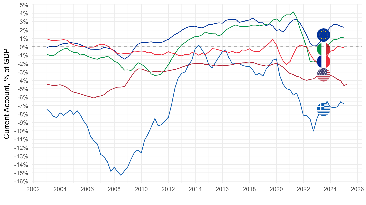

Greece, US, France

1999-

Quarterly

BOP |>
  filter(MEASURE == "CA",
         REF_AREA %in% c("FRA", "GRC", "USA"),
         FREQ == "Q",
         UNIT_MEASURE == "PT_B1GQ") |>
  quarter_to_date() |>
  
  arrange(desc(date)) |>
  mutate(Ref_area = ifelse(REF_AREA == "EU27_2020", "Europe", Ref_area)) |>
  left_join(colors, by = c("Ref_area" = "country")) |>
  mutate(color = ifelse(REF_AREA == "USA", color2, color)) |>
  mutate(obsValue = obsValue/100) |>
  filter(date >= as.Date("1999-01-01")) |>
  
  #filter(date <= as.Date("2021-01-01")) %>%
  ggplot() + geom_line(aes(x = date, y = obsValue, color = color)) + 
  theme_minimal() + xlab("") + ylab("Current Account, % of GDP") +
  scale_color_identity() + add_2flags +
  scale_x_date(breaks = c(seq(1990, 2100, 2)) |> paste0("-01-01") |> as.Date(),
               labels = date_format("%Y")) +
  scale_y_continuous(breaks = 0.01*seq(-60, 60, 1),
                     labels = scales::percent_format(accuracy = 1)) +
  geom_hline(yintercept = 0, linetype = "dashed", color = "black") +
  geom_label(data = . %>% filter(date == max(date)),
             aes(x = date, y = obsValue, label = percent(obsValue), color = color))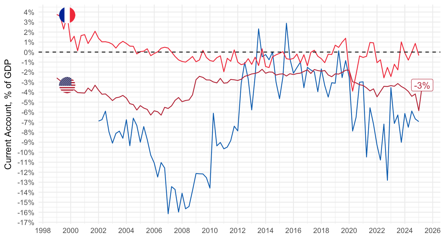

Smoothed

BOP |>
  filter(MEASURE == "CA",
         REF_AREA %in% c("FRA", "GRC", "USA"),
         FREQ == "Q",
         UNIT_MEASURE == "PT_B1GQ") |>
  quarter_to_date() |>
  
  arrange(desc(date)) |>
  mutate(Ref_area = ifelse(REF_AREA == "EU27_2020", "Europe", Ref_area)) |>
  left_join(colors, by = c("Ref_area" = "country")) |>
  mutate(color = ifelse(REF_AREA == "USA", color2, color)) |>
  mutate(obsValue = obsValue/100) |>
  group_by(REF_AREA) |>
  arrange(date) |>
  mutate(obsValue = zoo::rollmean(obsValue, k = 4, fill = NA, align = "right")) |>
  ungroup() |>
  filter(date >= as.Date("1999-01-01")) |>
  
  #filter(date <= as.Date("2021-01-01")) %>%
  ggplot() + geom_line(aes(x = date, y = obsValue, color = color)) + 
  theme_minimal() + xlab("") + ylab("Current Account, % of GDP") +
  scale_color_identity() + add_3flags +
  scale_x_date(breaks = c(seq(1990, 2100, 2)) |> paste0("-01-01") |> as.Date(),
               labels = date_format("%Y")) +
  scale_y_continuous(breaks = 0.01*seq(-60, 60, 1),
                     labels = scales::percent_format(accuracy = 1)) +
  geom_hline(yintercept = 0, linetype = "dashed", color = "black") +
  geom_label(data = . %>% filter(date == max(date)),
             aes(x = date, y = obsValue, label = percent(obsValue), color = color))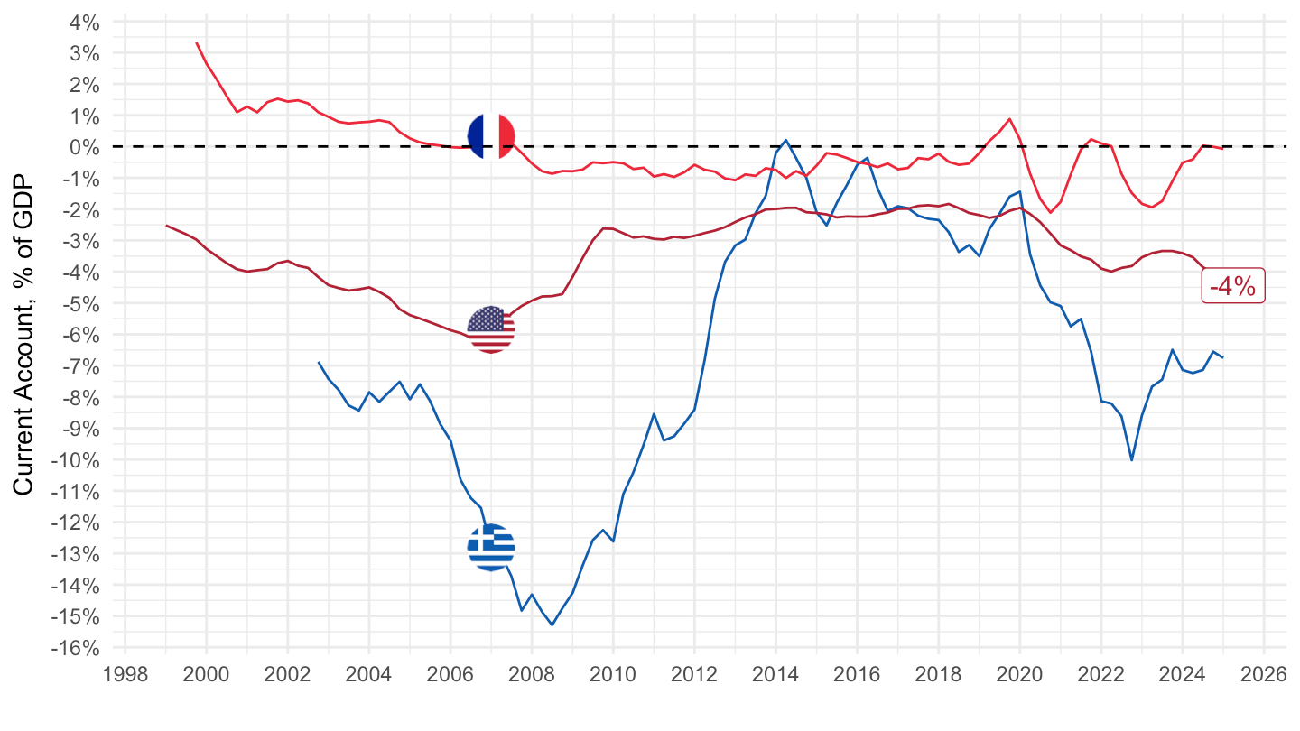

EU vs. US

All

BOP |>
  filter(MEASURE == "CA",
         REF_AREA %in% c("USA", "EA20"),
         FREQ == "Q",
         UNIT_MEASURE == "PT_B1GQ") |>
  quarter_to_date() |>
  
  arrange(desc(date)) |>
  mutate(Ref_area = ifelse(REF_AREA == "EA20", "Europe", Ref_area)) |>
  left_join(colors, by = c("Ref_area" = "country")) |>
  mutate(color = ifelse(REF_AREA == "USA", color2, color)) |>
  mutate(obsValue = obsValue/100) |>
  
  #filter(date <= as.Date("2021-01-01")) %>%
  ggplot() + geom_line(aes(x = date, y = obsValue, color = color)) + 
  theme_minimal() + xlab("") + ylab("Current Account, % of GDP") +
  scale_color_identity() + add_2flags +
  scale_x_date(breaks = seq(1920, 2100, 5) |> paste0("-01-01") |> as.Date(),
               labels = date_format("%Y")) +
  scale_y_continuous(breaks = 0.01*seq(-60, 60, 1),
                     labels = scales::percent_format(accuracy = 1)) +
  geom_hline(yintercept = 0, linetype = "dashed", color = "black")

2012-

BOP |>
  filter(MEASURE == "CA",
         REF_AREA %in% c("USA", "EA20"),
         FREQ == "Q",
         UNIT_MEASURE == "PT_B1GQ") |>
  quarter_to_date() |>
  
  arrange(desc(date)) |>
  mutate(Ref_area = ifelse(REF_AREA == "EA20", "Europe", Ref_area)) |>
  left_join(colors, by = c("Ref_area" = "country")) |>
  mutate(color = ifelse(REF_AREA == "USA", color2, color)) |>
  mutate(obsValue = obsValue/100) |>
  
  filter(date >= as.Date("2013-01-01")) |>
  ggplot() + geom_line(aes(x = date, y = obsValue, color = color)) + 
  theme_minimal() + xlab("") + ylab("Current Account, % of GDP") +
  scale_color_identity() + add_2flags +
  scale_x_date(breaks = seq(1920, 2100, 1) |> paste0("-01-01") |> as.Date(),
               labels = date_format("%Y")) +
  scale_y_continuous(breaks = 0.01*seq(-60, 60, 1),
                     labels = scales::percent_format(accuracy = 1)) +
  geom_hline(yintercept = 0, linetype = "dashed", color = "black")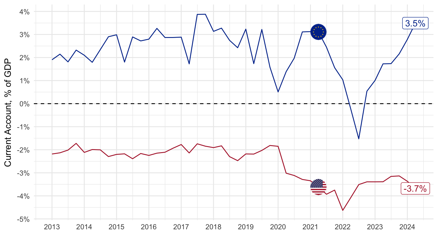

EU27_2020 vs. US

All

BOP |>
  filter(MEASURE == "CA",
         REF_AREA %in% c("USA", "EU27_2020"),
         FREQ == "Q",
         UNIT_MEASURE == "PT_B1GQ") |>
  quarter_to_date() |>
  
  arrange(desc(date)) |>
  mutate(Ref_area = ifelse(REF_AREA == "EU27_2020", "Europe", Ref_area)) |>
  left_join(colors, by = c("Ref_area" = "country")) |>
  mutate(color = ifelse(REF_AREA == "USA", color2, color)) |>
  mutate(obsValue = obsValue/100) |>
  
  #filter(date <= as.Date("2021-01-01")) %>%
  ggplot() + geom_line(aes(x = date, y = obsValue, color = color)) + 
  theme_minimal() + xlab("") + ylab("Current Account, % of GDP") +
  scale_color_identity() + add_2flags +
  scale_x_date(breaks = seq(1920, 2100, 5) |> paste0("-01-01") |> as.Date(),
               labels = date_format("%Y")) +
  scale_y_continuous(breaks = 0.01*seq(-60, 60, 1),
                     labels = scales::percent_format(accuracy = 1)) +
  geom_hline(yintercept = 0, linetype = "dashed", color = "black")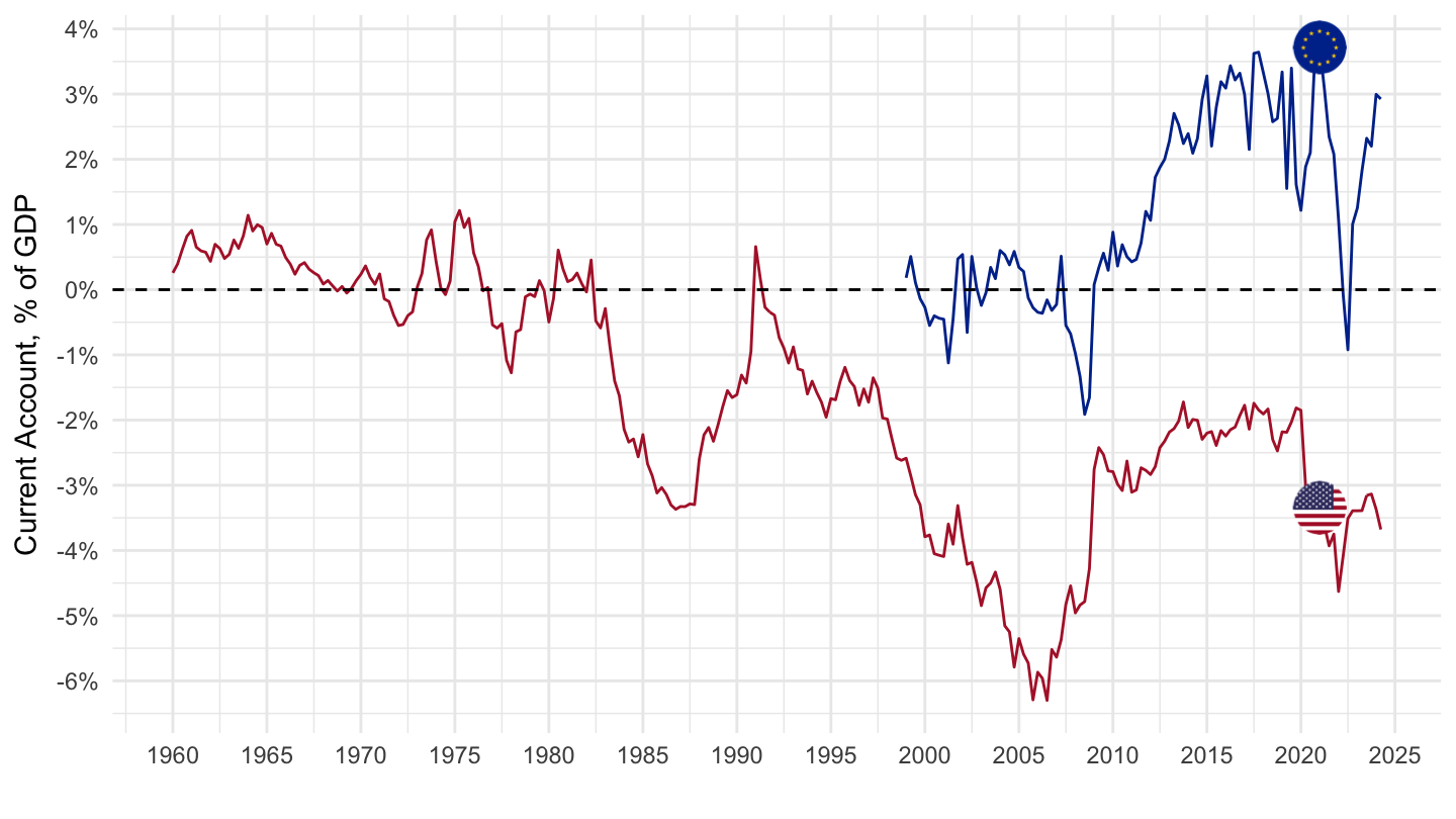

1999-

BOP |>
  filter(MEASURE == "CA",
         REF_AREA %in% c("USA", "EU27_2020"),
         FREQ == "Q",
         UNIT_MEASURE == "PT_B1GQ") |>
  quarter_to_date() |>
  
  arrange(desc(date)) |>
  mutate(Ref_area = ifelse(REF_AREA == "EU27_2020", "Europe", Ref_area)) |>
  left_join(colors, by = c("Ref_area" = "country")) |>
  mutate(color = ifelse(REF_AREA == "USA", color2, color)) |>
  mutate(obsValue = obsValue/100) |>
  filter(date >= as.Date("1999-01-01")) |>
  
  #filter(date <= as.Date("2021-01-01")) %>%
  ggplot() + geom_line(aes(x = date, y = obsValue, color = color)) + 
  theme_minimal() + xlab("") + ylab("Current Account, % of GDP") +
  scale_color_identity() + add_2flags +
  scale_x_date(breaks = c(seq(1990, 2100, 2)) |> paste0("-01-01") |> as.Date(),
               labels = date_format("%Y")) +
  scale_y_continuous(breaks = 0.01*seq(-60, 60, 1),
                     labels = scales::percent_format(accuracy = 1)) +
  geom_hline(yintercept = 0, linetype = "dashed", color = "black") +
  geom_label(data = . %>% filter(date == max(date)),
             aes(x = date, y = obsValue, label = percent(obsValue), color = color))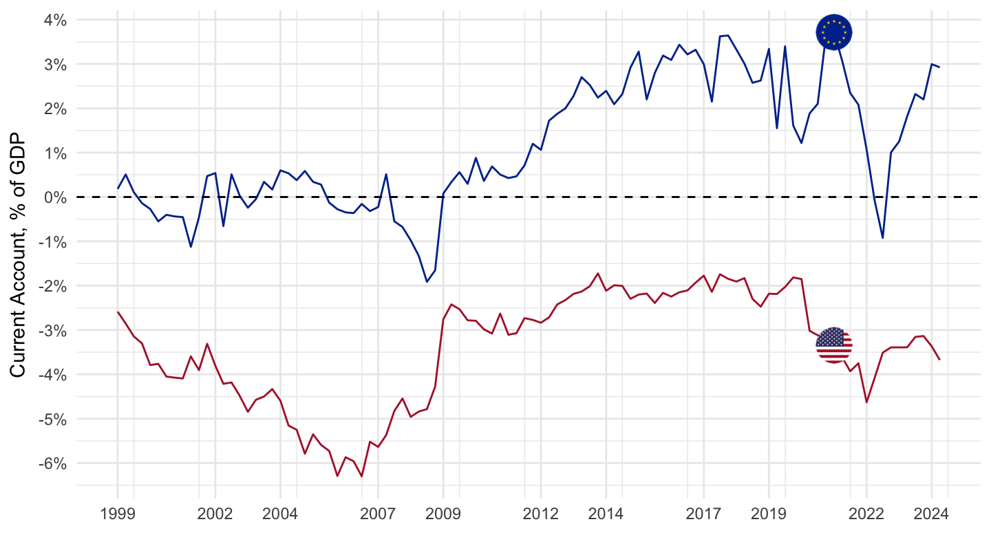

EU vs. US vs. IT

1999-

BOP |>
  filter(MEASURE == "CA",
         REF_AREA %in% c("USA", "EU27_2020", "ITA"),
         FREQ == "Q",
         UNIT_MEASURE == "PT_B1GQ") |>
  quarter_to_date() |>
  
  arrange(desc(date)) |>
  mutate(Ref_area = ifelse(REF_AREA == "EU27_2020", "Europe", Ref_area)) |>
  left_join(colors, by = c("Ref_area" = "country")) |>
  mutate(color = ifelse(REF_AREA == "USA", color2, color)) |>
  mutate(obsValue = obsValue/100) |>
  filter(date >= as.Date("1999-01-01")) |>
  
  #filter(date <= as.Date("2021-01-01")) %>%
  ggplot() + geom_line(aes(x = date, y = obsValue, color = color)) + 
  theme_minimal() + xlab("") + ylab("Current Account, % of GDP") +
  scale_color_identity() + add_3flags +
  scale_x_date(breaks = c(seq(1997, 2100, 5), seq(1999, 2100, 5)) |> paste0("-01-01") |> as.Date(),
               labels = date_format("%Y")) +
  scale_y_continuous(breaks = 0.01*seq(-60, 60, 1),
                     labels = scales::percent_format(accuracy = 1)) +
  geom_hline(yintercept = 0, linetype = "dashed", color = "black")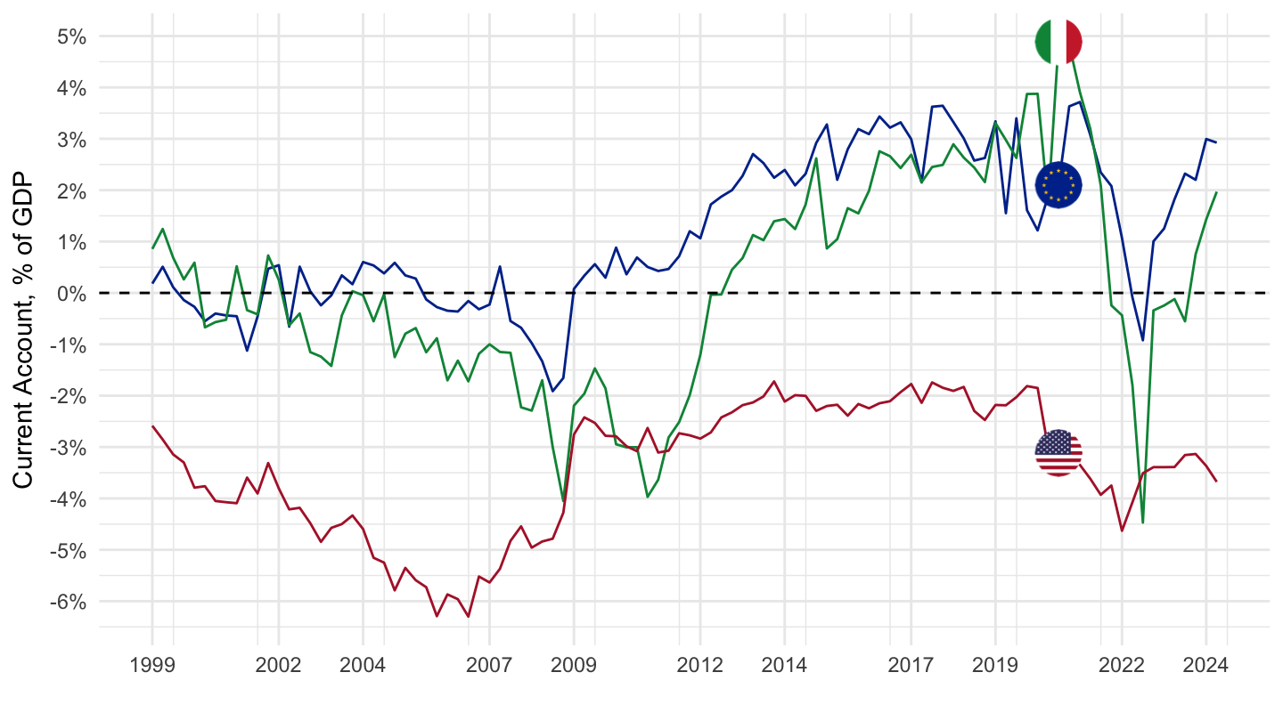

EU vs. US vs. DE vs. FR

All

BOP |>
  filter(MEASURE == "CA",
         REF_AREA %in% c("USA", "EU27_2020", "DEU", "FRA"),
         FREQ == "Q",
         UNIT_MEASURE == "PT_B1GQ") |>
  quarter_to_date() |>
  
  arrange(desc(date)) |>
  mutate(Ref_area = ifelse(REF_AREA == "EU27_2020", "Europe", Ref_area)) |>
  left_join(colors, by = c("Ref_area" = "country")) |>
  mutate(color = ifelse(REF_AREA == "USA", color2, color)) |>
  mutate(obsValue = obsValue/100) |>
  #filter(date >= as.Date("1999-01-01")) %>%
  
  #filter(date <= as.Date("2021-01-01")) %>%
  ggplot() + geom_line(aes(x = date, y = obsValue, color = color)) + 
  theme_minimal() + xlab("") + ylab("Current Account, % of GDP") +
  scale_color_identity() + add_4flags +
  scale_x_date(breaks = c(seq(1949, 2100, 5)) |> paste0("-01-01") |> as.Date(),
               labels = date_format("%Y")) +
  scale_y_continuous(breaks = 0.01*seq(-60, 60, 1),
                     labels = scales::percent_format(accuracy = 1)) +
  geom_hline(yintercept = 0, linetype = "dashed", color = "black")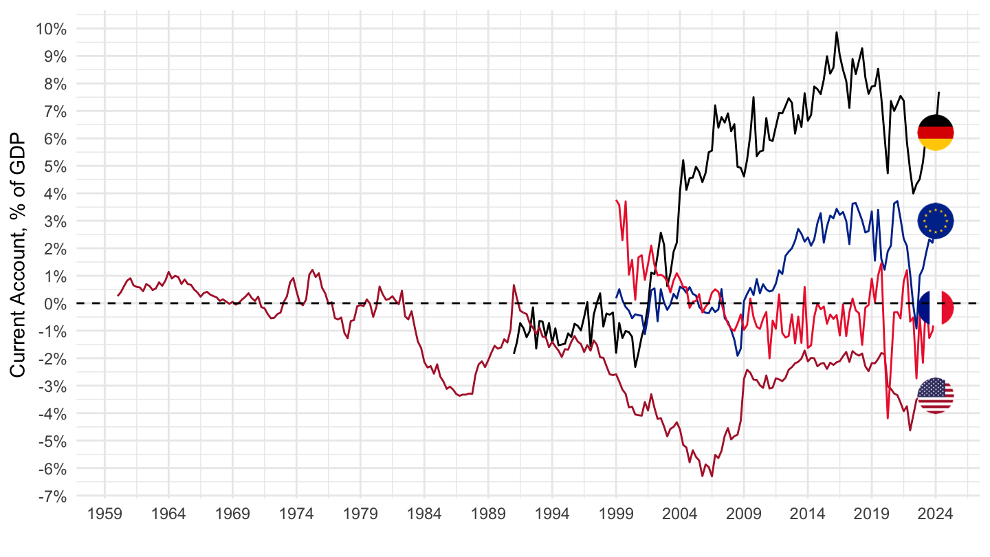

1999-

Quarterly

BOP |>
  filter(MEASURE == "CA",
         REF_AREA %in% c("USA", "EU27_2020", "DEU", "FRA"),
         FREQ == "Q",
         UNIT_MEASURE == "PT_B1GQ") |>
  quarter_to_date() |>
  
  arrange(desc(date)) |>
  mutate(Ref_area = ifelse(REF_AREA == "EU27_2020", "Europe", Ref_area)) |>
  left_join(colors, by = c("Ref_area" = "country")) |>
  mutate(color = ifelse(REF_AREA == "USA", color2, color)) |>
  mutate(obsValue = obsValue/100) |>
  filter(date >= as.Date("1999-01-01")) |>
  
  #filter(date <= as.Date("2021-01-01")) %>%
  ggplot() + geom_line(aes(x = date, y = obsValue, color = color)) + 
  theme_minimal() + xlab("") + ylab("Current Account, % of GDP") +
  scale_color_identity() + add_4flags +
  scale_x_date(breaks = c(seq(1997, 2100, 2)) |> paste0("-01-01") |> as.Date(),
               labels = date_format("%Y")) +
  scale_y_continuous(breaks = 0.01*seq(-60, 60, 1),
                     labels = scales::percent_format(accuracy = 1)) +
  geom_hline(yintercept = 0, linetype = "dashed", color = "black")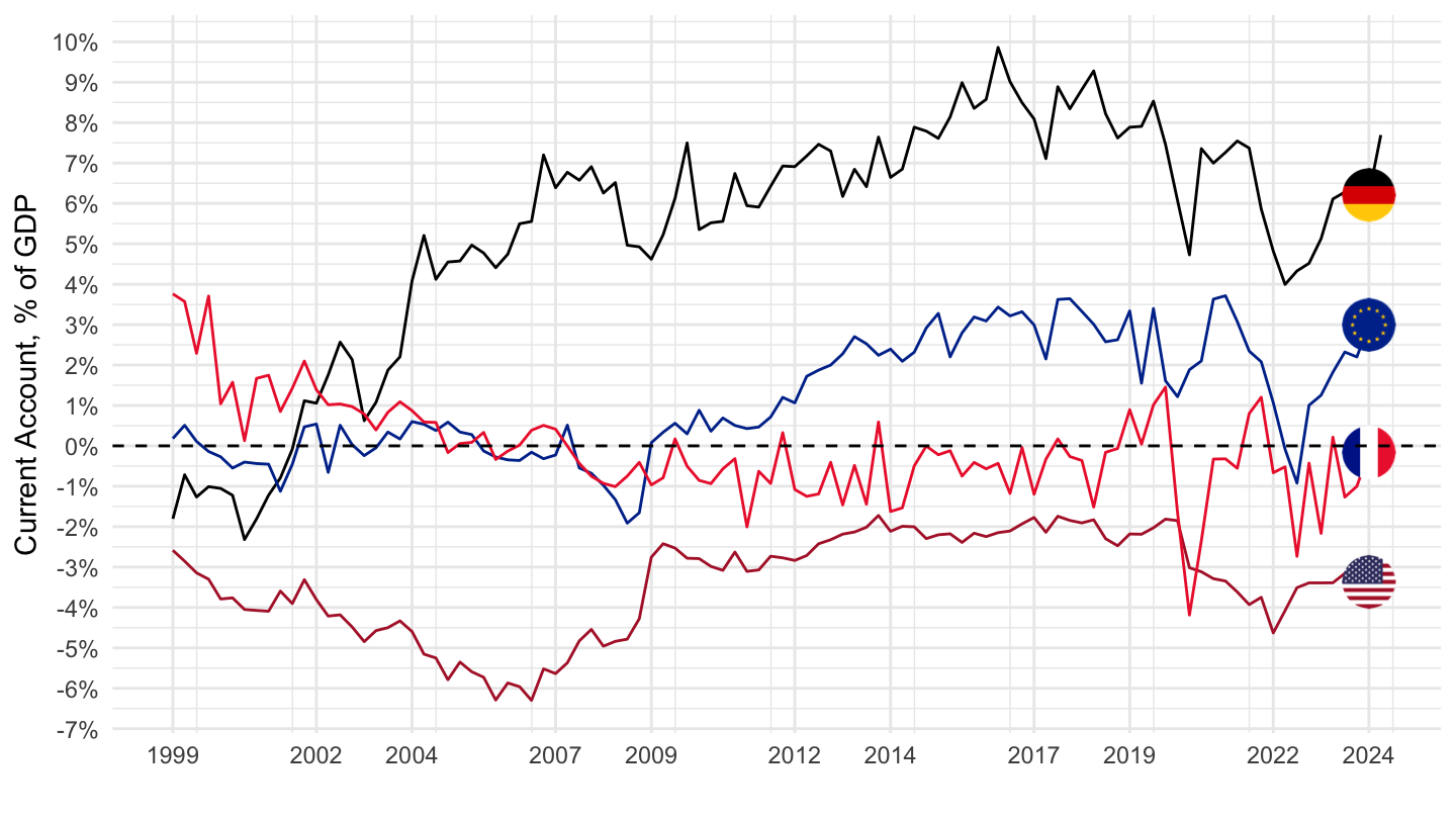

Smoothed

Quarterly

BOP |>
  filter(MEASURE == "CA",
         REF_AREA %in% c("USA", "EU27_2020", "DEU", "FRA"),
         FREQ == "Q",
         UNIT_MEASURE == "PT_B1GQ") |>
  quarter_to_date() |>
  
  arrange(desc(date)) |>
  mutate(Ref_area = ifelse(REF_AREA == "EU27_2020", "Europe", Ref_area)) |>
  left_join(colors, by = c("Ref_area" = "country")) |>
  mutate(color = ifelse(REF_AREA == "USA", color2, color)) |>
  mutate(obsValue = obsValue/100) |>
  filter(date >= as.Date("1999-01-01")) |>
  group_by(REF_AREA) |>
  arrange(date) |>
  mutate(obsValue_roll4 = zoo::rollmean(obsValue, k = 4, fill = NA, align = "right")) |>
  ungroup() |>
  
  #filter(date <= as.Date("2021-01-01")) %>%
  ggplot() + geom_line(aes(x = date, y = obsValue_roll4, color = color)) + 
  theme_minimal() + xlab("") + ylab("Current Account, % of GDP") +
  scale_color_identity() + add_4flags +
  scale_x_date(breaks = c(seq(1997, 2100, 2)) |> paste0("-01-01") |> as.Date(),
               labels = date_format("%Y")) +
  scale_y_continuous(breaks = 0.01*seq(-60, 60, 1),
                     labels = scales::percent_format(accuracy = 1)) +
  geom_hline(yintercept = 0, linetype = "dashed", color = "black")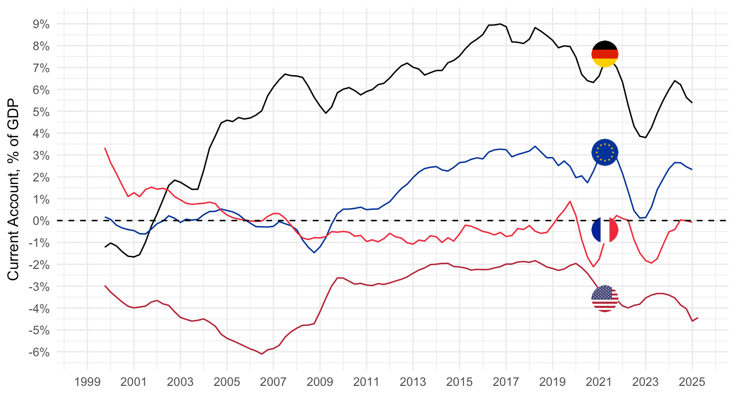

EU vs. US vs. DE

All

BOP |>
  filter(MEASURE == "CA",
         REF_AREA %in% c("USA", "EU27_2020", "DEU"),
         FREQ == "Q",
         UNIT_MEASURE == "PT_B1GQ") |>
  quarter_to_date() |>
  
  arrange(desc(date)) |>
  mutate(Ref_area = ifelse(REF_AREA == "EU27_2020", "Europe", Ref_area)) |>
  left_join(colors, by = c("Ref_area" = "country")) |>
  mutate(color = ifelse(REF_AREA == "USA", color2, color)) |>
  mutate(obsValue = obsValue/100) |>
  #filter(date >= as.Date("1999-01-01")) %>%
  
  #filter(date <= as.Date("2021-01-01")) %>%
  ggplot() + geom_line(aes(x = date, y = obsValue, color = color)) + 
  theme_minimal() + xlab("") + ylab("Current Account, % of GDP") +
  scale_color_identity() + add_4flags +
  scale_x_date(breaks = c(seq(1949, 2100, 5)) |> paste0("-01-01") |> as.Date(),
               labels = date_format("%Y")) +
  scale_y_continuous(breaks = 0.01*seq(-60, 60, 1),
                     labels = scales::percent_format(accuracy = 1)) +
  geom_hline(yintercept = 0, linetype = "dashed", color = "black")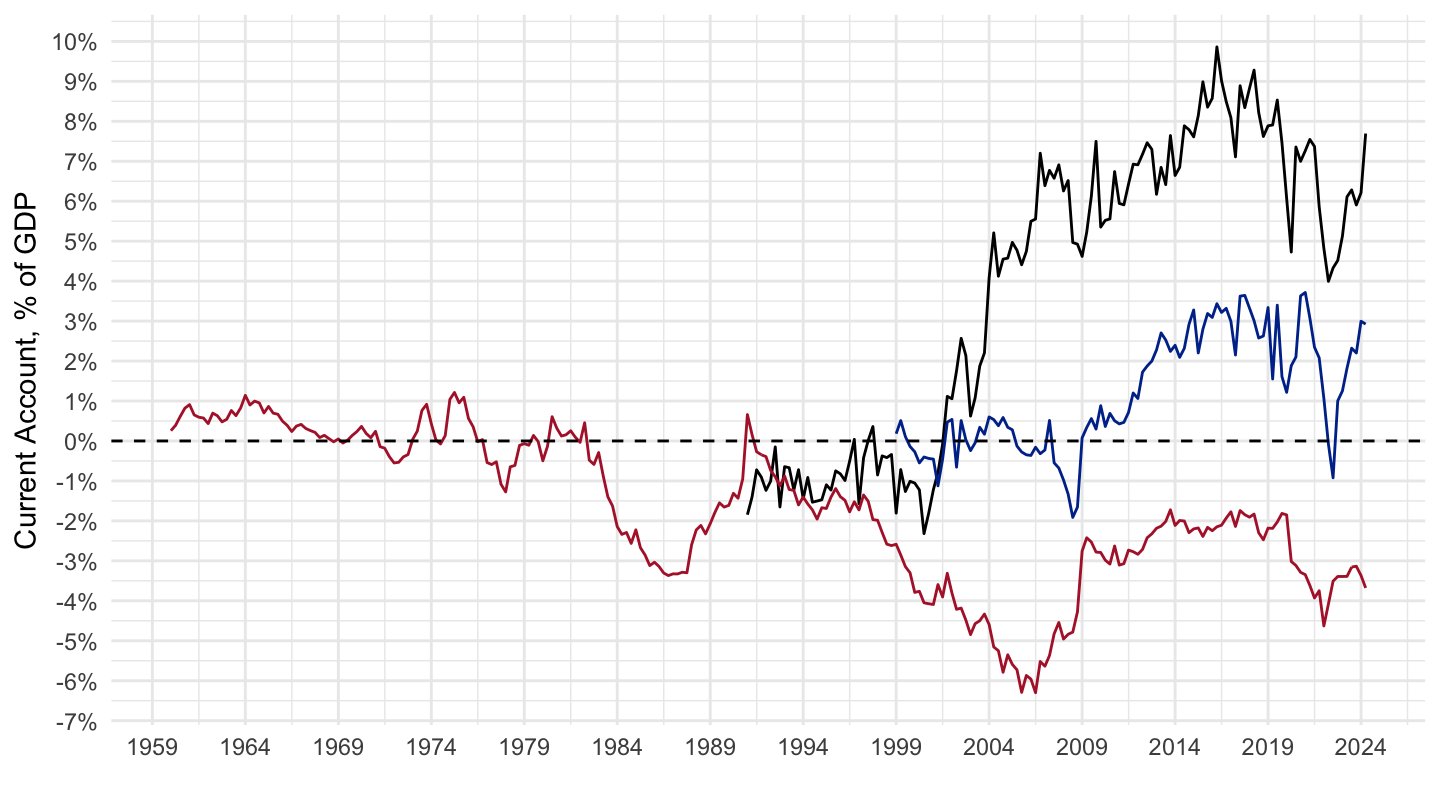

1999-

BOP |>
  filter(MEASURE == "CA",
         REF_AREA %in% c("USA", "EU27_2020", "DEU"),
         FREQ == "Q",
         UNIT_MEASURE == "PT_B1GQ") |>
  quarter_to_date() |>
  
  arrange(desc(date)) |>
  mutate(Ref_area = ifelse(REF_AREA == "EU27_2020", "Europe", Ref_area)) |>
  left_join(colors, by = c("Ref_area" = "country")) |>
  mutate(color = ifelse(REF_AREA == "USA", color2, color)) |>
  mutate(obsValue = obsValue/100) |>
  filter(date >= as.Date("1999-01-01")) |>
  
  #filter(date <= as.Date("2021-01-01")) %>%
  ggplot() + geom_line(aes(x = date, y = obsValue, color = color)) + 
  theme_minimal() + xlab("") + ylab("Current Account, % of GDP") +
  scale_color_identity() + add_3flags +
  scale_x_date(breaks = c(seq(1997, 2100, 5), seq(1999, 2100, 5)) |> paste0("-01-01") |> as.Date(),
               labels = date_format("%Y")) +
  scale_y_continuous(breaks = 0.01*seq(-60, 60, 1),
                     labels = scales::percent_format(accuracy = 1)) +
  geom_hline(yintercept = 0, linetype = "dashed", color = "black")