
Last observation: Q2 2026 (N = 52) · 2025 (N = 123)
First observation: 1948 (N = 1) · Q1 1975 (N = 1)
Last data update: 06 oct. 2026, 18:15
Last compile: 09 oct. 2026, 22:47
IFR_BP6_USD |>
  group_by(FREQ) |>
  summarise(Nobs = n()) |>
  arrange(-Nobs) |>
print_table_conditional()| FREQ | Nobs |
|---|---|
| Q | 10119 |
| A | 4390 |
IFR_BP6_USD |>
  left_join(REF_AREA, by = "REF_AREA") |>
  group_by(REF_AREA, Ref_area) |>
  summarise(Nobs = n()) |>
  arrange(-Nobs) |>
  mutate(Flag = gsub(" ", "-", str_to_lower(gsub(" ", "-", Ref_area))),
         Flag = paste0('<img src="../../icon/flag/round/vsmall/', Flag, '.png" alt="Flag">')) |>
  select(Flag, everything()) %>%
{if (is_html_output()) datatable(., filter = 'top', rownames = F, escape = F) else .}IFR_BP6_USD |>
filter(FREQ == "A",
TIME_PERIOD %in% c("2018", "2019", "2020")) |>
left_join(REF_AREA, by = "REF_AREA") |>
select(REF_AREA, Ref_area, TIME_PERIOD, OBS_VALUE) |>
spread(TIME_PERIOD, OBS_VALUE) |>
filter(abs(`2018`) > 10000, `2018` < 0) |>
arrange(`2018`) %>%
mutate_at(vars(-1, -2), funs(round(./1000))) |>
mutate(Flag = gsub(" ", "-", str_to_lower(gsub(" ", "-", Ref_area))),
Flag = paste0('<img src="../../icon/flag/round/vsmall/', Flag, '.png" alt="Flag">')) |>
select(Flag, everything()) %>%
{if (is_html_output()) datatable(., filter = 'top', rownames = F, escape = F) else .}IFR_BP6_USD |>
filter(FREQ == "A",
TIME_PERIOD %in% c("2016", "2019", "2013", "2010", "2007")) |>
left_join(REF_AREA, by = "REF_AREA") |>
select(REF_AREA, Ref_area, TIME_PERIOD, OBS_VALUE) |>
spread(TIME_PERIOD, OBS_VALUE) |>
filter(abs(`2019`) > 10000, `2019` > 0) |>
arrange(-`2019`) %>%
mutate_at(vars(-1, -2), funs(round(./1000))) |>
mutate(Flag = gsub(" ", "-", str_to_lower(gsub(" ", "-", Ref_area))),
Flag = paste0('<img src="../../icon/flag/round/vsmall/', Flag, '.png" alt="Flag">')) |>
select(Flag, everything()) %>%
{if (is_html_output()) datatable(., filter = 'top', rownames = F, escape = F) else .}i_g("bib/imf/IFR_BP6_USD_ex1.png")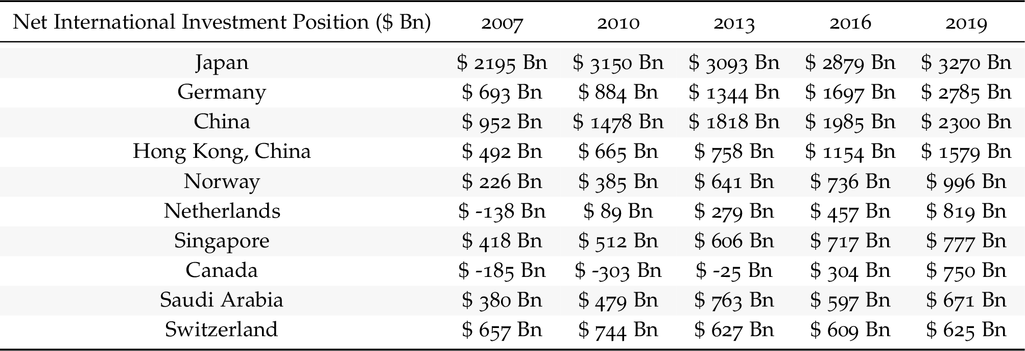
IFR_BP6_USD |>
  filter(FREQ == "A",
         TIME_PERIOD %in% c("2018", "2019", "2020")) |>
  left_join(REF_AREA, by = "REF_AREA") |>
  select(REF_AREA, Ref_area, TIME_PERIOD, OBS_VALUE) |>
  spread(TIME_PERIOD, OBS_VALUE) |>
  arrange(-`2018`) %>%
  mutate_at(vars(-1, -2), funs(round(./1000))) |>
  mutate(Flag = gsub(" ", "-", str_to_lower(gsub(" ", "-", Ref_area))),
         Flag = paste0('<img src="../../icon/flag/round/vsmall/', Flag, '.png" alt="Flag">')) |>
  select(Flag, everything()) %>%
{if (is_html_output()) datatable(., filter = 'top', rownames = F, escape = F) else .}IFR_BP6_USD |>
filter(FREQ == "A",
REF_AREA %in% c("DE", "FR", "IT", "ES")) |>
year_to_date2() |>
select(date, OBS_VALUE, REF_AREA) |>
left_join(REF_AREA, by = "REF_AREA") |>
mutate(OBS_VALUE = OBS_VALUE/1000,
Counterpart_area = Ref_area) |>
add_flag_color("Counterpart_area") |>
ggplot() + scale_color_identity() + theme_minimal() +
geom_line(aes(x = date, y = OBS_VALUE, color = color)) +
theme(legend.title = element_blank(),
legend.position = c(0.2, 0.8)) +
scale_x_date(breaks = seq(1950, 2100, 5) |> paste0("-01-01") |> as.Date(),
labels = date_format("%Y")) +
add_flags +
scale_y_continuous(breaks = scales::breaks_pretty(n = 10),
labels = dollar_format(accuracy = 1, suffix = " Bn", prefix = "$")) +
xlab("") + ylab("Net International Investment Positions")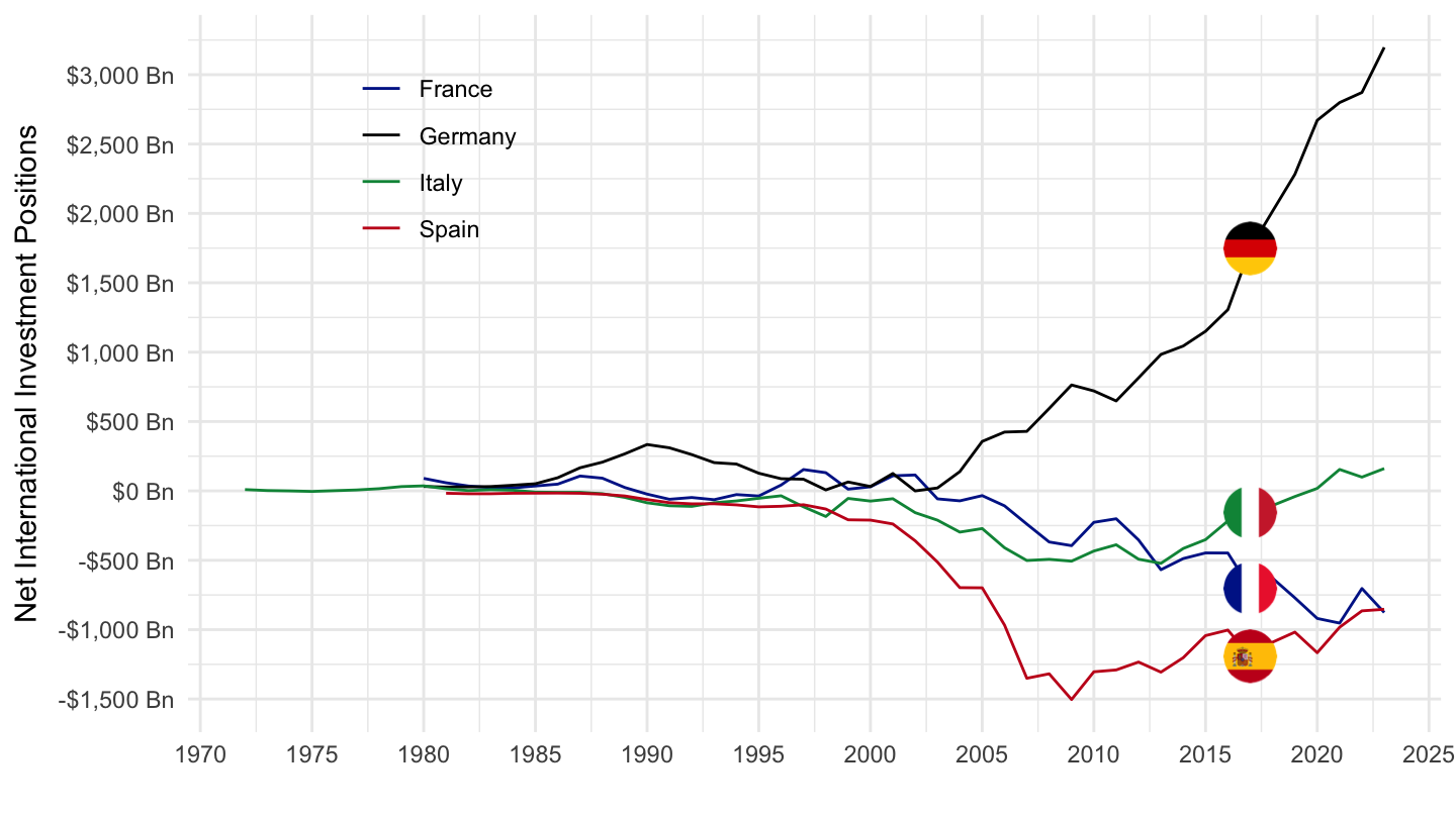
IFR_BP6_USD |>
  filter(FREQ == "A",
         REF_AREA %in% c("DE", "FR", "US")) |>
  year_to_date2() |>
  select(date, OBS_VALUE, REF_AREA) |>
  left_join(REF_AREA, by = "REF_AREA") |>
    mutate(OBS_VALUE = OBS_VALUE/1000) |>
  add_flag_color("Ref_area") |>
ggplot() + scale_color_identity() + add_flags + theme_minimal() +
  geom_line(aes(x = date, y = OBS_VALUE, color = color)) +
  theme(legend.title = element_blank(),
        legend.position = c(0.2, 0.4)) +
  scale_x_date(breaks = seq(1950, 2100, 5) |> paste0("-01-01") |> as.Date(),
               labels = date_format("%Y")) +
  scale_y_continuous(breaks = scales::breaks_pretty(n = 10),
                     labels = dollar_format(accuracy = 1, suffix = " Bn", prefix = "$")) +
  xlab("") + ylab("Net International Investment Positions")
IFR_BP6_USD |>
  filter(FREQ == "A",
         TIME_PERIOD == "2019") |>
  select(REF_AREA, OBS_VALUE) |>
  left_join(NY.GDP.MKTP.CD |>
              filter(year == 2019) |>
              select(REF_AREA = iso2c, NY.GDP.MKTP.CD = value),
            by = c("REF_AREA")) |>
  mutate(`IIP (% of GDP)` = (10^6)*OBS_VALUE/NY.GDP.MKTP.CD) |>
  left_join(REF_AREA, by = "REF_AREA") |>
  select(REF_AREA, Ref_area, `IIP (% of GDP)`) |>
  arrange(`IIP (% of GDP)`) |>
  mutate(`IIP (% of GDP)` = round(100*`IIP (% of GDP)`)) |>
  mutate(Flag = gsub(" ", "-", str_to_lower(gsub(" ", "-", Ref_area))),
         Flag = paste0('<img src="../../icon/flag/round/vsmall/', Flag, '.png" alt="Flag">')) |>
  select(Flag, everything()) %>%
{if (is_html_output()) datatable(., filter = 'top', rownames = F, escape = F) else .}IFR_BP6_USD |>
filter(FREQ == "A",
TIME_PERIOD == "2019") |>
select(REF_AREA, OBS_VALUE) |>
left_join(NY.GDP.MKTP.CD |>
filter(year == 2019) |>
select(REF_AREA = iso2c, NY.GDP.MKTP.CD = value),
by = c("REF_AREA")) |>
mutate(`IIP (% of GDP)` = (10^6)*OBS_VALUE/NY.GDP.MKTP.CD) |>
left_join(REF_AREA, by = "REF_AREA") |>
select(REF_AREA, Ref_area, `IIP (% of GDP)`) |>
arrange(`IIP (% of GDP)`) |>
mutate(`IIP (% of GDP)` = round(100*`IIP (% of GDP)`)) |>
head(30) |>
mutate(Flag = gsub(" ", "-", str_to_lower(gsub(" ", "-", Ref_area))),
Flag = paste0('<img src="../../icon/flag/round/vsmall/', Flag, '.png" alt="Flag">')) |>
select(Flag, everything()) %>%
{if (is_html_output()) datatable(., filter = 'top', rownames = F, escape = F) else .}IFR_BP6_USD |>
filter(FREQ == "A",
TIME_PERIOD == "2019") |>
select(REF_AREA, OBS_VALUE) |>
left_join(NY.GDP.MKTP.CD |>
filter(year == 2019) |>
select(REF_AREA = iso2c, NY.GDP.MKTP.CD = value),
by = c("REF_AREA")) |>
mutate(`IIP (% of GDP)` = (10^6)*OBS_VALUE/NY.GDP.MKTP.CD) |>
left_join(REF_AREA, by = "REF_AREA") |>
select(REF_AREA, Ref_area, `IIP (% of GDP)`) |>
arrange(-`IIP (% of GDP)`) |>
mutate(`IIP (% of GDP)` = round(100*`IIP (% of GDP)`)) |>
head(30) |>
mutate(Flag = gsub(" ", "-", str_to_lower(gsub(" ", "-", Ref_area))),
Flag = paste0('<img src="../../icon/flag/round/vsmall/', Flag, '.png" alt="Flag">')) |>
select(Flag, everything()) %>%
{if (is_html_output()) datatable(., filter = 'top', rownames = F, escape = F) else .}IFR_BP6_USD |>
filter(FREQ == "A",
REF_AREA %in% c("PH", "TH", "ID")) |>
year_to_date2() |>
select(date, OBS_VALUE, REF_AREA) |>
left_join(NY.GDP.MKTP.CD |>
mutate(date = as.Date(paste0(year, "-01-01"))) |>
select(REF_AREA = iso2c, date, NY.GDP.MKTP.CD = value),
by = c("REF_AREA", "date")) |>
mutate(value = (10^6)*OBS_VALUE/NY.GDP.MKTP.CD) |>
select(-OBS_VALUE) |>
left_join(REF_AREA, by = "REF_AREA") |>
add_flag_color("Ref_area") |>
ggplot() + add_flags + theme_minimal() + scale_color_identity() +
geom_line(aes(x = date, y = value, color = color)) +
theme(legend.title = element_blank(),
legend.position = c(0.2, 0.85)) +
scale_x_date(breaks = seq(1950, 2100, 5) |> paste0("-01-01") |> as.Date(),
labels = date_format("%Y")) +
scale_y_continuous(breaks = 0.01*seq(-300, 200, 10),
labels = scales::percent_format(accuracy = 1)) +
xlab("") + ylab("Net International Investment Position (% of GDP)")
IFR_BP6_USD |>
  filter(FREQ == "A",
         REF_AREA %in% c("US", "ES", "DE", "FR", "GR", "IT")) |>
  year_to_date2() |>
  select(date, OBS_VALUE, REF_AREA) |>
  left_join(NY.GDP.MKTP.CD |>
              mutate(date = as.Date(paste0(year, "-01-01"))) |>
              select(REF_AREA = iso2c, date, NY.GDP.MKTP.CD = value),
            by = c("REF_AREA", "date")) |>
  mutate(value = (10^6)*OBS_VALUE/NY.GDP.MKTP.CD) |>
  left_join(REF_AREA, by = "REF_AREA") |>
  add_flag_color("Ref_area") |>
  mutate(Counterpart_area = Ref_area,
         OBS_VALUE = value) |>
  ggplot() + theme_minimal() + scale_color_identity() +
  geom_line(aes(x = date, y = OBS_VALUE, color = color)) +
  theme(legend.title = element_blank(),
        legend.position = c(0.2, 0.85)) +
  scale_x_date(breaks = seq(1950, 2100, 5) |> paste0("-01-01") |> as.Date(),
               labels = date_format("%Y")) +
  add_flags +
  scale_y_continuous(breaks = 0.01*seq(-300, 200, 20),
                     labels = scales::percent_format(accuracy = 1)) +
  xlab("") + ylab("Net International Investment Position\n% of GDP") +
  geom_hline(yintercept = 0, linetype = "dashed")
IFR_BP6_USD |>
  filter(FREQ == "A",
         REF_AREA %in% c("AR", "UY", "CL", "PE")) |>
  year_to_date2() |>
  select(date, OBS_VALUE, REF_AREA) |>
  left_join(NY.GDP.MKTP.CD |>
              mutate(date = as.Date(paste0(year, "-01-01"))) |>
              select(REF_AREA = iso2c, date, NY.GDP.MKTP.CD = value),
            by = c("REF_AREA", "date")) |>
  mutate(value = (10^6)*OBS_VALUE/NY.GDP.MKTP.CD) |>
  select(-OBS_VALUE) |>
  left_join(REF_AREA, by = "REF_AREA") |>
  add_flag_color("Ref_area") |>
  ggplot() + add_flags + theme_minimal() + scale_color_identity() +
  geom_line(aes(x = date, y = value, color = color)) +
  theme(legend.title = element_blank(),
        legend.position = c(0.2, 0.85)) +
  scale_x_date(breaks = seq(1950, 2100, 5) |> paste0("-01-01") |> as.Date(),
               labels = date_format("%Y")) +
  scale_y_continuous(breaks = 0.01*seq(-300, 200, 10),
                     labels = scales::percent_format(accuracy = 1)) +
  xlab("") + ylab("Net International Investment Position (% of GDP)")
IFR_BP6_USD |>
  filter(FREQ == "A",
         REF_AREA %in% c("SE", "AT", "NL", "DE")) |>
  year_to_date2() |>
  select(date, OBS_VALUE, REF_AREA) |>
  left_join(NY.GDP.MKTP.CD |>
              mutate(date = as.Date(paste0(year, "-01-01"))) |>
              select(REF_AREA = iso2c, date, NY.GDP.MKTP.CD = value),
            by = c("REF_AREA", "date")) |>
  mutate(value = (10^6)*OBS_VALUE/NY.GDP.MKTP.CD) |>
  select(-OBS_VALUE) |>
  left_join(REF_AREA, by = "REF_AREA") |>
    add_flag_color("Ref_area") |>
ggplot() + scale_color_identity() + add_flags + theme_minimal() +
  geom_line(aes(x = date, y = value, color = color)) +
  theme(legend.title = element_blank(),
        legend.position = c(0.2, 0.85)) +
  scale_x_date(breaks = seq(1950, 2100, 5) |> paste0("-01-01") |> as.Date(),
               labels = date_format("%Y")) +
  scale_y_continuous(breaks = 0.01*seq(-300, 200, 10),
                     labels = scales::percent_format(accuracy = 1)) +
  xlab("") + ylab("Net International Investment Position (% of GDP)")
IFR_BP6_USD |>
  filter(FREQ == "A",
         REF_AREA %in% c("FR", "ES", "PT", "IT", "DE")) |>
  year_to_date2() |>
  filter(date >= as.Date("1980-01-01")) |>
  select(date, OBS_VALUE, REF_AREA) |>
  left_join(NY.GDP.MKTP.CD |>
              mutate(date = as.Date(paste0(year, "-01-01"))) |>
              select(REF_AREA = iso2c, date, NY.GDP.MKTP.CD = value),
            by = c("REF_AREA", "date")) |>
  mutate(value = (10^6)*OBS_VALUE/NY.GDP.MKTP.CD) |>
  select(-OBS_VALUE) |>
  left_join(REF_AREA, by = "REF_AREA") |>
  add_flag_color("Ref_area") |>
  ggplot() + add_flags + theme_minimal() +
  geom_line(aes(x = date, y = value, color = color)) +
  theme(legend.position = "none") + scale_color_identity() +
  scale_x_date(breaks = seq(1950, 2100, 5) |> paste0("-01-01") |> as.Date(),
               labels = date_format("%Y")) +
  scale_y_continuous(breaks = 0.01*seq(-300, 200, 10),
                     labels = scales::percent_format(accuracy = 1)) +
  xlab("") + ylab("Net International Investment Position (% of GDP)") +
  geom_hline(yintercept = 0, linetype = "dashed", color = "grey")
IFR_BP6_USD |>
  filter(FREQ == "A",
         REF_AREA %in% c("FR", "GR", "ES", "PT")) |>
  year_to_date2() |>
  select(date, OBS_VALUE, REF_AREA) |>
  left_join(NY.GDP.MKTP.CD |>
              mutate(date = as.Date(paste0(year, "-01-01"))) |>
              select(REF_AREA = iso2c, date, NY.GDP.MKTP.CD = value),
            by = c("REF_AREA", "date")) |>
  mutate(value = (10^6)*OBS_VALUE/NY.GDP.MKTP.CD) |>
  select(-OBS_VALUE) |>
  left_join(REF_AREA, by = "REF_AREA") |>
    add_flag_color("Ref_area") |>
ggplot() + scale_color_identity() + add_flags + theme_minimal() +
  geom_line(aes(x = date, y = value, color = color)) +
  theme(legend.position = "none") +
  scale_x_date(breaks = seq(1950, 2100, 5) |> paste0("-01-01") |> as.Date(),
               labels = date_format("%Y")) +
  scale_y_continuous(breaks = 0.01*seq(-300, 200, 10),
                     labels = scales::percent_format(accuracy = 1)) +
  xlab("") + ylab("Net International Investment Position (% of GDP)") +
  geom_hline(yintercept = 0, linetype = "dashed", color = "grey")
IFR_BP6_USD |>
  filter(FREQ == "A",
         REF_AREA %in% c("FR", "CA", "US", "DE", "IT", "JP", "GB")) |>
  year_to_date2() |>
  select(date, OBS_VALUE, REF_AREA) |>
  left_join(NY.GDP.MKTP.CD |>
              mutate(date = as.Date(paste0(year, "-01-01"))) |>
              select(REF_AREA = iso2c, date, NY.GDP.MKTP.CD = value),
            by = c("REF_AREA", "date")) |>
  mutate(value = (10^6)*OBS_VALUE/NY.GDP.MKTP.CD) |>
  select(-OBS_VALUE) |>
  left_join(REF_AREA, by = "REF_AREA") |>
  na.omit() |>
    add_flag_color("Ref_area") |>
ggplot() + scale_color_identity() + add_flags + theme_minimal() +
  geom_line(aes(x = date, y = value, color = color)) +
  theme(legend.position = "none") +
  scale_x_date(breaks = seq(1950, 2100, 5) |> paste0("-01-01") |> as.Date(),
               labels = date_format("%Y")) +
  scale_y_continuous(breaks = 0.01*seq(-300, 200, 10),
                     labels = scales::percent_format(accuracy = 1)) +
  xlab("") + ylab("Net International Investment Position (% of GDP)") +
  geom_hline(yintercept = 0, linetype = "dashed", color = "grey")
IFR_BP6_USD |>
  filter(FREQ == "A",
         REF_AREA %in% c("FR", "CA", "US", "DE", "IT", "JP", "GB")) |>
  year_to_date2() |>
  select(date, OBS_VALUE, REF_AREA) |>
  left_join(NY.GDP.MKTP.CD |>
              mutate(date = as.Date(paste0(year, "-01-01"))) |>
              select(REF_AREA = iso2c, date, NY.GDP.MKTP.CD = value),
            by = c("REF_AREA", "date")) |>
  mutate(value = (10^6)*OBS_VALUE/NY.GDP.MKTP.CD) |>
  select(-OBS_VALUE) |>
  left_join(REF_AREA, by = "REF_AREA") |>
  filter(date >= as.Date("1980-01-01")) |>
  na.omit() |>
    add_flag_color("Ref_area") |>
ggplot() + scale_color_identity() + add_flags + theme_minimal() +
  geom_line(aes(x = date, y = value, color = color)) +
  theme(legend.position = "none") +
  scale_x_date(breaks = seq(1950, 2100, 5) |> paste0("-01-01") |> as.Date(),
               labels = date_format("%Y")) +
  scale_y_continuous(breaks = 0.01*seq(-300, 200, 10),
                     labels = scales::percent_format(accuracy = 1)) +
  xlab("") + ylab("Net International Investment Position (% of GDP)") +
  geom_hline(yintercept = 0, linetype = "dashed", color = "grey")
IFR_BP6_USD |>
  filter(FREQ == "A",
         REF_AREA %in% c("FR", "CA", "US", "DE", "IT", "JP", "GB")) |>
  year_to_date2() |>
  select(date, OBS_VALUE, REF_AREA) |>
  left_join(NY.GDP.MKTP.CD |>
              mutate(date = as.Date(paste0(year, "-01-01"))) |>
              select(REF_AREA = iso2c, date, NY.GDP.MKTP.CD = value),
            by = c("REF_AREA", "date")) |>
  mutate(value = (10^6)*OBS_VALUE/NY.GDP.MKTP.CD) |>
  select(-OBS_VALUE) |>
  left_join(REF_AREA, by = "REF_AREA") |>
  filter(date >= as.Date("2000-01-01")) |>
  na.omit() |>
    add_flag_color("Ref_area") |>
ggplot() + scale_color_identity() + add_flags + theme_minimal() +
  geom_line(aes(x = date, y = value, color = color)) +
  theme(legend.position = "none") +
  scale_x_date(breaks = seq(1950, 2100, 2) |> paste0("-01-01") |> as.Date(),
               labels = date_format("%Y")) +
  scale_y_continuous(breaks = 0.01*seq(-300, 200, 10),
                     labels = scales::percent_format(accuracy = 1)) +
  xlab("") + ylab("Net International Investment Position (% of GDP)") +
  geom_hline(yintercept = 0, linetype = "dashed", color = "grey")
IFR_BP6_USD |>
  filter(FREQ == "A",
         REF_AREA %in% c("FR", "GR", "ES", "PT", "US")) |>
  year_to_date2() |>
  select(date, OBS_VALUE, REF_AREA) |>
  left_join(NY.GDP.MKTP.CD |>
              mutate(date = as.Date(paste0(year, "-01-01"))) |>
              select(REF_AREA = iso2c, date, NY.GDP.MKTP.CD = value),
            by = c("REF_AREA", "date")) |>
  mutate(value = (10^6)*OBS_VALUE/NY.GDP.MKTP.CD) |>
  select(-OBS_VALUE) |>
  left_join(REF_AREA, by = "REF_AREA") |>
    add_flag_color("Ref_area") |>
ggplot() + scale_color_identity() + add_flags + theme_minimal() +
  geom_line(aes(x = date, y = value, color = color)) +
  theme(legend.position = "none") +
  scale_x_date(breaks = seq(1950, 2100, 5) |> paste0("-01-01") |> as.Date(),
               labels = date_format("%Y")) +
  scale_y_continuous(breaks = 0.01*seq(-300, 200, 10),
                     labels = scales::percent_format(accuracy = 1)) +
  xlab("") + ylab("Net International Investment Position (% of GDP)") +
  geom_hline(yintercept = 0, linetype = "dashed", color = "grey")
IFR_BP6_USD |>
  filter(FREQ == "A",
         REF_AREA %in% c("FR", "DE", "GR", "ES", "PT", "US", "GB", "NL")) |>
  year_to_date2() |>
  select(date, OBS_VALUE, REF_AREA) |>
  left_join(NY.GDP.MKTP.CD |>
              mutate(date = as.Date(paste0(year, "-01-01"))) |>
              select(REF_AREA = iso2c, date, NY.GDP.MKTP.CD = value),
            by = c("REF_AREA", "date")) |>
  mutate(value = (10^6)*OBS_VALUE/NY.GDP.MKTP.CD) |>
  select(-OBS_VALUE) |>
  left_join(REF_AREA, by = "REF_AREA") |>
    add_flag_color("Ref_area") |>
ggplot() + scale_color_identity() + add_flags + theme_minimal() +
  geom_line(aes(x = date, y = value, color = color)) +
  theme(legend.position = "none") +
  scale_x_date(breaks = seq(1950, 2100, 5) |> paste0("-01-01") |> as.Date(),
               labels = date_format("%Y")) +
  scale_y_continuous(breaks = 0.01*seq(-300, 200, 10),
                     labels = scales::percent_format(accuracy = 1)) +
  xlab("") + ylab("Net International Investment Position (% of GDP)") +
  geom_hline(yintercept = 0, linetype = "dashed", color = "grey")
IFR_BP6_USD |>
  filter(FREQ == "A",
         REF_AREA %in% c("US", "GB", "AU", "NZ")) |>
  year_to_date2() |>
  select(date, OBS_VALUE, REF_AREA) |>
  left_join(NY.GDP.MKTP.CD |>
              mutate(date = as.Date(paste0(year, "-01-01"))) |>
              select(REF_AREA = iso2c, date, NY.GDP.MKTP.CD = value),
            by = c("REF_AREA", "date")) |>
  mutate(value = (10^6)*OBS_VALUE/NY.GDP.MKTP.CD) |>
  select(-OBS_VALUE) |>
  left_join(REF_AREA, by = "REF_AREA") |>
    add_flag_color("Ref_area") |>
ggplot() + scale_color_identity() + add_flags + theme_minimal() +
  geom_line(aes(x = date, y = value, color = color)) +
  theme(legend.position = "none") +
  scale_x_date(breaks = seq(1950, 2100, 5) |> paste0("-01-01") |> as.Date(),
               labels = date_format("%Y")) +
  scale_y_continuous(breaks = 0.01*seq(-300, 200, 10),
                     labels = scales::percent_format(accuracy = 1)) +
  xlab("") + ylab("Net International Investment Position (% of GDP)")
IFR_BP6_USD |>
  filter(FREQ == "A",
         REF_AREA %in% c("US", "GB", "AU", "NZ", "FR")) |>
  year_to_date2() |>
  select(date, OBS_VALUE, REF_AREA) |>
  left_join(NY.GDP.MKTP.CD |>
              mutate(date = as.Date(paste0(year, "-01-01"))) |>
              select(REF_AREA = iso2c, date, NY.GDP.MKTP.CD = value),
            by = c("REF_AREA", "date")) |>
  mutate(value = (10^6)*OBS_VALUE/NY.GDP.MKTP.CD) |>
  select(-OBS_VALUE) |>
  left_join(REF_AREA, by = "REF_AREA") |>
    add_flag_color("Ref_area") |>
ggplot() + scale_color_identity() + add_flags + theme_minimal() +
  geom_line(aes(x = date, y = value, color = color)) +
  theme(legend.position = "none") +
  scale_x_date(breaks = seq(1950, 2100, 5) |> paste0("-01-01") |> as.Date(),
               labels = date_format("%Y")) +
  scale_y_continuous(breaks = 0.01*seq(-300, 200, 10),
                     labels = scales::percent_format(accuracy = 1)) +
  xlab("") + ylab("Net International Investment Position (% of GDP)") +
  geom_hline(yintercept = 0, linetype = "dashed", color = "grey")
IFR_BP6_USD |>
  filter(FREQ == "A",
         REF_AREA %in% c("U2", "US", "JP")) |>
  mutate(OBS_VALUE = OBS_VALUE*(10^(UNIT_MULT))) |>
  year_to_date2() |>
  filter(date >= as.Date("1995-01-01")) |>
  select(date, INDICATOR, OBS_VALUE, REF_AREA) |>
  mutate(REF_AREA = ifelse(REF_AREA == "U2", "XC", REF_AREA)) |>
  # Match U2 = Euro area (Member States and Institutions of the Euro Area) changing composition with XC in WDI
  left_join(NY.GDP.MKTP.CD |>
              mutate(date = as.Date(paste0(year, "-01-01"))) |>
              select(REF_AREA = iso2c, date, NY.GDP.MKTP.CD = value),
            by = c("REF_AREA", "date")) |>
  mutate(value = OBS_VALUE/NY.GDP.MKTP.CD) |>
  select(-OBS_VALUE) |>
  left_join(REF_AREA, by = "REF_AREA") |>
  mutate(Ref_area = case_when(REF_AREA == "XC" ~ "Europe",
                              T ~ Ref_area)) |>
    add_flag_color("Ref_area") |>
ggplot() + scale_color_identity() + add_flags + theme_minimal() +
  geom_line(aes(x = date, y = value, color = color)) +
  theme(legend.position = "none") +
  scale_x_date(breaks = seq(1950, 2100, 5) |> paste0("-01-01") |> as.Date(),
               labels = date_format("%Y")) +
  scale_y_continuous(breaks = 0.01*seq(-300, 200, 5),
                     labels = scales::percent_format(accuracy = 1)) +
  xlab("") + ylab("Net International Investment Position (% of GDP)") +
  geom_hline(yintercept = 0, linetype = "dashed", color = "grey")
IFR_BP6_USD |>
  filter(FREQ == "A",
         REF_AREA %in% c("U2", "US")) |>
  mutate(OBS_VALUE = OBS_VALUE*(10^(UNIT_MULT))) |>
  year_to_date2() |>
  filter(date >= as.Date("1995-01-01")) |>
  select(date, INDICATOR, OBS_VALUE, REF_AREA) |>
  mutate(REF_AREA = ifelse(REF_AREA == "U2", "XC", REF_AREA)) |>
  # Match U2 = Euro area (Member States and Institutions of the Euro Area) changing composition with XC in WDI
  left_join(NY.GDP.MKTP.CD |>
              mutate(date = as.Date(paste0(year, "-01-01"))) |>
              select(REF_AREA = iso2c, date, NY.GDP.MKTP.CD = value),
            by = c("REF_AREA", "date")) |>
  mutate(value = OBS_VALUE/NY.GDP.MKTP.CD) |>
  select(-OBS_VALUE) |>
  left_join(REF_AREA, by = "REF_AREA") |>
  mutate(Ref_area = case_when(REF_AREA == "XC" ~ "Europe",
                              T ~ Ref_area)) |>
    add_flag_color("Ref_area") |>
ggplot() + scale_color_identity() + add_flags + theme_minimal() +
  geom_line(aes(x = date, y = value, color = color)) +
  theme(legend.position = "none") +
  scale_x_date(breaks = seq(1950, 2100, 2) |> paste0("-01-01") |> as.Date(),
               labels = date_format("%Y")) +
  scale_y_continuous(breaks = 0.01*seq(-300, 200, 5),
                     labels = scales::percent_format(accuracy = 1)) +
  xlab("") + ylab("Net International Investment Position (% of GDP)") +
  geom_hline(yintercept = 0, linetype = "dashed", color = "grey")
IFR_BP6_USD |>
  filter(FREQ == "A",
         REF_AREA %in% c("U2", "US")) |>
  mutate(OBS_VALUE = OBS_VALUE*(10^(UNIT_MULT))) |>
  year_to_date2() |>
  filter(date >= as.Date("1999-01-01")) |>
  select(date, INDICATOR, OBS_VALUE, REF_AREA) |>
  mutate(REF_AREA = ifelse(REF_AREA == "U2", "XC", REF_AREA)) |>
  # Match U2 = Euro area (Member States and Institutions of the Euro Area) changing composition with XC in WDI
  left_join(NY.GDP.MKTP.CD |>
              mutate(date = as.Date(paste0(year, "-01-01"))) |>
              select(REF_AREA = iso2c, date, NY.GDP.MKTP.CD = value),
            by = c("REF_AREA", "date")) |>
  mutate(value = OBS_VALUE/NY.GDP.MKTP.CD) |>
  select(-OBS_VALUE) |>
  left_join(REF_AREA, by = "REF_AREA") |>
  mutate(Ref_area = case_when(REF_AREA == "XC" ~ "Europe",
                              T ~ Ref_area)) |>
    add_flag_color("Ref_area") |>
ggplot() + scale_color_identity() + add_flags + theme_minimal() +
  geom_line(aes(x = date, y = value, color = color)) +
  theme(legend.position = "none") +
  scale_x_date(breaks = seq(1950, 2100, 2) |> paste0("-01-01") |> as.Date(),
               labels = date_format("%Y")) +
  scale_y_continuous(breaks = 0.01*seq(-300, 200, 5),
                     labels = scales::percent_format(accuracy = 1)) +
  xlab("") + ylab("Net International Investment Position (% of GDP)") +
  geom_hline(yintercept = 0, linetype = "dashed", color = "black")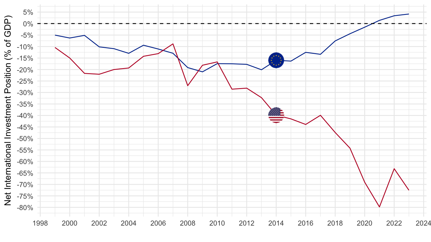
IFR_BP6_USD |>
  bind_rows(NGDP_USD) |>
  filter(FREQ == "A",
         REF_AREA %in% c("U2", "US")) |>
  mutate(OBS_VALUE = OBS_VALUE*(10^(UNIT_MULT))) |>
  year_to_date2() |>
  filter(date >= as.Date("1995-01-01")) |>
  select(date, INDICATOR, OBS_VALUE, REF_AREA) |>
  spread(INDICATOR, OBS_VALUE) |>
  mutate(value = IFR_BP6_USD/NGDP_USD) |>
  left_join(REF_AREA, by = "REF_AREA") |>
  mutate(Ref_area = case_when(REF_AREA == "U2" ~ "Europe",
                              T ~ Ref_area)) |>
    add_flag_color("Ref_area") |>
ggplot() + scale_color_identity() + add_flags + theme_minimal() +
  geom_line(aes(x = date, y = value, color = color)) +
  theme(legend.position = "none") +
  scale_x_date(breaks = seq(1950, 2100, 5) |> paste0("-01-01") |> as.Date(),
               labels = date_format("%Y")) +
  scale_y_continuous(breaks = 0.01*seq(-300, 200, 5),
                     labels = scales::percent_format(accuracy = 1)) +
  xlab("") + ylab("Net International Investment Position (% of GDP)")
IFR_BP6_USD |>
  bind_rows(NGDP_USD) |>
  filter(FREQ == "A",
         REF_AREA %in% c("U2", "US", "CN")) |>
  mutate(OBS_VALUE = OBS_VALUE*(10^(UNIT_MULT))) |>
  year_to_date2() |>
  filter(date >= as.Date("1995-01-01")) |>
  select(date, INDICATOR, OBS_VALUE, REF_AREA) |>
  spread(INDICATOR, OBS_VALUE) |>
  mutate(value = IFR_BP6_USD/NGDP_USD) |>
  left_join(REF_AREA, by = "REF_AREA") |>
  mutate(Ref_area = case_when(REF_AREA == "CN" ~ "China",
                              REF_AREA == "U2" ~ "Europe",
                              T ~ Ref_area)) |>
    add_flag_color("Ref_area") |>
ggplot() + scale_color_identity() + add_flags + theme_minimal() +
  geom_line(aes(x = date, y = value, color = color)) +
  theme(legend.position = "none") +
  scale_x_date(breaks = seq(1950, 2100, 5) |> paste0("-01-01") |> as.Date(),
               labels = date_format("%Y")) +
  scale_y_continuous(breaks = 0.01*seq(-300, 200, 5),
                     labels = scales::percent_format(accuracy = 1)) +
  xlab("") + ylab("Net International Investment Position (% of GDP)")
IFR_BP6_USD |>
  filter(FREQ == "A",
         REF_AREA %in% c("SE", "AT", "NL", "DK")) |>
  year_to_date2() |>
  select(date, OBS_VALUE, REF_AREA) |>
  left_join(NY.GDP.MKTP.CD |>
              mutate(date = as.Date(paste0(year, "-01-01"))) |>
              select(REF_AREA = iso2c, date, NY.GDP.MKTP.CD = value),
            by = c("REF_AREA", "date")) |>
  mutate(value = (10^6)*OBS_VALUE/NY.GDP.MKTP.CD) |>
  select(-OBS_VALUE) |>
  left_join(REF_AREA, by = "REF_AREA") |>
    add_flag_color("Ref_area") |>
ggplot() + scale_color_identity() + add_flags + theme_minimal() + geom_line(aes(x = date, y = value, color = color)) +
  theme(legend.title = element_blank(),
        legend.position = c(0.2, 0.85)) +
  scale_x_date(breaks = seq(1950, 2100, 5) |> paste0("-01-01") |> as.Date(),
               labels = date_format("%Y")) +
  scale_y_continuous(breaks = 0.01*seq(-300, 60, 10),
                     labels = scales::percent_format(accuracy = 1)) +
  xlab("") + ylab("Net International Investment Position (% of GDP)")
IFR_BP6_USD |>
  filter(`FREQ` == "A",
         `REF_AREA` %in% c("LB", "GR", "AR")) |>
  year_to_date2() |>
  select(date, OBS_VALUE, REF_AREA) |>
  left_join(NY.GDP.MKTP.CD |>
              mutate(date = as.Date(paste0(year, "-01-01"))) |>
              select(REF_AREA = iso2c, date, NY.GDP.MKTP.CD = value),
            by = c("REF_AREA", "date")) |>
  mutate(value = (10^6)*OBS_VALUE/NY.GDP.MKTP.CD) |>
  select(-OBS_VALUE) |>
  left_join(REF_AREA, by = "REF_AREA") |>
    add_flag_color("Ref_area") |>
ggplot() + scale_color_identity() + add_flags + theme_minimal() + geom_line(aes(x = date, y = value, color = color)) +
  theme(legend.title = element_blank(),
        legend.position = c(0.2, 0.8)) +
  scale_x_date(breaks = seq(1950, 2100, 5) |> paste0("-01-01") |> as.Date(),
               labels = date_format("%Y")) +
  scale_y_continuous(breaks = 0.01*seq(-60, 60, 10),
                     labels = scales::percent_format(accuracy = 1)) +
  xlab("") + ylab("Net International Investment Position (% of GDP)")
IFR_BP6_USD |>
  filter(`FREQ` == "A",
         `REF_AREA` %in% c("DE", "FR", "IT")) |>
  year_to_date2() |>
  select(date, OBS_VALUE, REF_AREA) |>
  left_join(NY.GDP.MKTP.CD |>
              mutate(date = as.Date(paste0(year, "-01-01"))) |>
              select(REF_AREA = iso2c, date, NY.GDP.MKTP.CD = value),
            by = c("REF_AREA", "date")) |>
  mutate(value = (10^6)*OBS_VALUE/NY.GDP.MKTP.CD) |>
  select(-OBS_VALUE) |>
  left_join(REF_AREA, by = "REF_AREA") |>
    add_flag_color("Ref_area") |>
ggplot() + scale_color_identity() + add_flags + theme_minimal() +
  geom_line(aes(x = date, y = value, color = color)) +
  theme(legend.title = element_blank(),
        legend.position = c(0.2, 0.8)) +
  scale_x_date(breaks = seq(1950, 2100, 5) |> paste0("-01-01") |> as.Date(),
               labels = date_format("%Y")) +
  scale_y_continuous(breaks = 0.01*seq(-60, 60, 10),
                     labels = scales::percent_format(accuracy = 1)) +
  xlab("") + ylab("Net International Investment Position (% of GDP)")
IFR_BP6_USD |>
  filter(`FREQ` == "A",
         `REF_AREA` %in% c("GR", "ES", "PT")) |>
  year_to_date2() |>
  select(date, OBS_VALUE, REF_AREA) |>
  left_join(NY.GDP.MKTP.CD |>
              mutate(date = as.Date(paste0(year, "-01-01"))) |>
              select(REF_AREA = iso2c, date, NY.GDP.MKTP.CD = value),
            by = c("REF_AREA", "date")) |>
  mutate(value = (10^6)*OBS_VALUE/NY.GDP.MKTP.CD) |>
  select(-OBS_VALUE) |>
  left_join(REF_AREA, by = "REF_AREA") |>
    add_flag_color("Ref_area") |>
ggplot() + scale_color_identity() + add_flags + theme_minimal() + geom_line(aes(x = date, y = value, color = color)) +
  theme(legend.title = element_blank(),
        legend.position = c(0.2, 0.2)) +
  scale_x_date(breaks = seq(1950, 2100, 5) |> paste0("-01-01") |> as.Date(),
               labels = date_format("%Y")) +
  scale_y_continuous(breaks = 0.01*seq(-300, 60, 10),
                     labels = scales::percent_format(accuracy = 1)) +
  xlab("") + ylab("Net International Investment Position (% of GDP)")
IFR_BP6_USD |>
  filter(`FREQ` == "A",
         `REF_AREA` %in% c("DE", "JP", "NL")) |>
  year_to_date2() |>
  select(date, OBS_VALUE, REF_AREA) |>
  left_join(NY.GDP.MKTP.CD |>
              mutate(date = as.Date(paste0(year, "-01-01"))) |>
              select(REF_AREA = iso2c, date, NY.GDP.MKTP.CD = value),
            by = c("REF_AREA", "date")) |>
  mutate(value = (10^6)*OBS_VALUE/NY.GDP.MKTP.CD) |>
  select(-OBS_VALUE) |>
  left_join(REF_AREA, by = "REF_AREA") |>
    add_flag_color("Ref_area") |>
ggplot() + scale_color_identity() + add_flags + theme_minimal() + geom_line(aes(x = date, y = value, color = color)) +
  theme(legend.title = element_blank(),
        legend.position = c(0.2, 0.8)) +
  scale_x_date(breaks = seq(1950, 2100, 5) |> paste0("-01-01") |> as.Date(),
               labels = date_format("%Y")) +
  scale_y_continuous(breaks = 0.01*seq(-100, 100, 10),
                     labels = scales::percent_format(accuracy = 1)) +
  xlab("") + ylab("Net International Investment Position (% of GDP)")
IFR_BP6_USD |>
  filter(`FREQ` == "A",
         `REF_AREA` %in% c("CH", "NO", "DK")) |>
  year_to_date2() |>
  select(date, OBS_VALUE, REF_AREA) |>
  left_join(NY.GDP.MKTP.CD |>
              mutate(date = as.Date(paste0(year, "-01-01"))) |>
              select(REF_AREA = iso2c, date, NY.GDP.MKTP.CD = value),
            by = c("REF_AREA", "date")) |>
  mutate(value = (10^6)*OBS_VALUE/NY.GDP.MKTP.CD) |>
  select(-OBS_VALUE) |>
  left_join(REF_AREA, by = "REF_AREA") |>
    add_flag_color("Ref_area") |>
ggplot() + scale_color_identity() + add_flags + theme_minimal() + geom_line(aes(x = date, y = value, color = color)) +
  theme(legend.title = element_blank(),
        legend.position = c(0.2, 0.8)) +
  scale_x_date(breaks = seq(1950, 2100, 5) |> paste0("-01-01") |> as.Date(),
               labels = date_format("%Y")) +
  scale_y_continuous(breaks = 0.01*seq(-100, 300, 20),
                     labels = scales::percent_format(accuracy = 1)) +
  xlab("") + ylab("Net International Investment Position (% of GDP)")
IFR_BP6_USD |>
  filter(`FREQ` == "A",
         `REF_AREA` %in% c("BH", "KW", "SA")) |>
  year_to_date2() |>
  select(date, OBS_VALUE, REF_AREA) |>
  left_join(NY.GDP.MKTP.CD |>
              mutate(date = as.Date(paste0(year, "-01-01"))) |>
              select(REF_AREA = iso2c, date, NY.GDP.MKTP.CD = value),
            by = c("REF_AREA", "date")) |>
  mutate(value = (10^6)*OBS_VALUE/NY.GDP.MKTP.CD) |>
  select(-OBS_VALUE) |>
  left_join(REF_AREA, by = "REF_AREA") |>
    add_flag_color("Ref_area") |>
ggplot() + scale_color_identity() + add_flags + theme_minimal() + geom_line(aes(x = date, y = value, color = color)) +
  theme(legend.title = element_blank(),
        legend.position = c(0.2, 0.8)) +
  scale_x_date(breaks = seq(1950, 2100, 5) |> paste0("-01-01") |> as.Date(),
               labels = date_format("%Y")) +
  scale_y_continuous(breaks = 0.01*seq(-100, 300, 10),
                     labels = scales::percent_format(accuracy = 1)) +
  xlab("") + ylab("Net International Investment Position (% of GDP)")
IFR_BP6_USD |>
  filter(`FREQ` == "A",
         `REF_AREA` %in% c("HU", "MX", "AU")) |>
  year_to_date2() |>
  select(date, OBS_VALUE, REF_AREA) |>
  left_join(NY.GDP.MKTP.CD |>
              mutate(date = as.Date(paste0(year, "-01-01"))) |>
              select(REF_AREA = iso2c, date, NY.GDP.MKTP.CD = value),
            by = c("REF_AREA", "date")) |>
  mutate(value = (10^6)*OBS_VALUE/NY.GDP.MKTP.CD) |>
  select(-OBS_VALUE) |>
  left_join(REF_AREA, by = "REF_AREA") |>
    add_flag_color("Ref_area") |>
ggplot() + scale_color_identity() + add_flags + theme_minimal() + geom_line(aes(x = date, y = value, color = color)) +
  theme(legend.title = element_blank(),
        legend.position = c(0.2, 0.2)) +
  scale_x_date(breaks = seq(1950, 2100, 5) |> paste0("-01-01") |> as.Date(),
               labels = date_format("%Y")) +
  scale_y_continuous(breaks = 0.01*seq(-200, 300, 10),
                     labels = scales::percent_format(accuracy = 1)) +
  xlab("") + ylab("Net International Investment Position (% of GDP)")
IFR_BP6_USD |>
  filter(`FREQ` == "A",
         `REF_AREA` %in% c("FI", "SE", "AR")) |>
  year_to_date2() |>
  select(date, OBS_VALUE, REF_AREA) |>
  left_join(NY.GDP.MKTP.CD |>
              mutate(date = as.Date(paste0(year, "-01-01"))) |>
              select(REF_AREA = iso2c, date, NY.GDP.MKTP.CD = value),
            by = c("REF_AREA", "date")) |>
  mutate(value = (10^6)*OBS_VALUE/NY.GDP.MKTP.CD) |>
  select(-OBS_VALUE) |>
  left_join(REF_AREA, by = "REF_AREA") |>
    add_flag_color("Ref_area") |>
ggplot() + scale_color_identity() + add_flags + theme_minimal() + geom_line(aes(x = date, y = value, color = color)) +
  theme(legend.title = element_blank(),
        legend.position = c(0.2, 0.2)) +
  scale_x_date(breaks = seq(1950, 2100, 5) |> paste0("-01-01") |> as.Date(),
               labels = date_format("%Y")) +
  scale_y_continuous(breaks = 0.01*seq(-600, 300, 20),
                     labels = scales::percent_format(accuracy = 1)) +
  xlab("") + ylab("Net International Investment Position (% of GDP)")
IFR_BP6_USD |>
  filter(`FREQ` == "A",
         `REF_AREA` %in% c("KR", "ID", "TH")) |>
  year_to_date2() |>
  select(date, OBS_VALUE, REF_AREA) |>
  left_join(NY.GDP.MKTP.CD |>
              mutate(date = as.Date(paste0(year, "-01-01"))) |>
              select(REF_AREA = iso2c, date, NY.GDP.MKTP.CD = value),
            by = c("REF_AREA", "date")) |>
  mutate(value = (10^6)*OBS_VALUE/NY.GDP.MKTP.CD) |>
  select(-OBS_VALUE) |>
  left_join(REF_AREA, by = "REF_AREA") |>
    add_flag_color("Ref_area") |>
ggplot() + scale_color_identity() + add_flags + theme_minimal() + geom_line(aes(x = date, y = value, color = color)) +
  theme(legend.title = element_blank(),
        legend.position = c(0.2, 0.85)) +
  scale_x_date(breaks = seq(1950, 2100, 5) |> paste0("-01-01") |> as.Date(),
               labels = date_format("%Y")) +
  scale_y_continuous(breaks = 0.01*seq(-600, 300, 20),
                     labels = scales::percent_format(accuracy = 1)) +
  xlab("") + ylab("Net International Investment Position (% of GDP)")
IFR_BP6_USD |>
  filter(`FREQ` == "A",
         `REF_AREA` %in% c("PH", "SG", "MY")) |>
  year_to_date2() |>
  select(date, OBS_VALUE, REF_AREA) |>
  left_join(NY.GDP.MKTP.CD |>
              mutate(date = as.Date(paste0(year, "-01-01"))) |>
              select(REF_AREA = iso2c, date, NY.GDP.MKTP.CD = value),
            by = c("REF_AREA", "date")) |>
  mutate(value = (10^6)*OBS_VALUE/NY.GDP.MKTP.CD) |>
  select(-OBS_VALUE) |>
  left_join(REF_AREA, by = "REF_AREA") |>
    add_flag_color("Ref_area") |>
ggplot() + scale_color_identity() + add_flags + theme_minimal() + geom_line(aes(x = date, y = value, color = color)) +
  theme(legend.title = element_blank(),
        legend.position = c(0.2, 0.85)) +
  scale_x_date(breaks = seq(1950, 2100, 5) |> paste0("-01-01") |> as.Date(),
               labels = date_format("%Y")) +
  scale_y_continuous(breaks = 0.01*seq(-600, 300, 20),
                     labels = scales::percent_format(accuracy = 1)) +
  xlab("") + ylab("Net International Investment Position (% of GDP)")
IFR_BP6_USD |>
  filter(`FREQ` == "A",
         `REF_AREA` %in% c("CL", "UY", "TR")) |>
  year_to_date2() |>
  select(date, OBS_VALUE, REF_AREA) |>
  left_join(NY.GDP.MKTP.CD |>
              mutate(date = as.Date(paste0(year, "-01-01"))) |>
              select(REF_AREA = iso2c, date, NY.GDP.MKTP.CD = value),
            by = c("REF_AREA", "date")) |>
  mutate(value = (10^6)*OBS_VALUE/NY.GDP.MKTP.CD) |>
  select(-OBS_VALUE) |>
  left_join(REF_AREA, by = "REF_AREA") |>
    add_flag_color("Ref_area") |>
ggplot() + scale_color_identity() + add_flags + theme_minimal() + geom_line(aes(x = date, y = value, color = color)) +
  theme(legend.title = element_blank(),
        legend.position = c(0.2, 0.85)) +
  scale_x_date(breaks = seq(1950, 2100, 5) |> paste0("-01-01") |> as.Date(),
               labels = date_format("%Y")) +
  scale_y_continuous(breaks = 0.01*seq(-600, 300, 10),
                     labels = scales::percent_format(accuracy = 1)) +
  xlab("") + ylab("Net International Investment Position (% of GDP)")
| source | dataset | Title | Updated |
|---|---|---|---|
| source | dataset | Title | Updated |
|---|---|---|---|


