Unemployment by sex and age – quarterly data
Data - Eurostat
Info
Last observation: Quarterly: 2026Q1 (N = 6,804)
First observation: Quarterly: 2003Q1 (N = 189)
Last data update: 23 jul 2026, 22:44. Last compile: 24 jul 2026, 04:09
Structure
France, Germany, Portugal
All
Code
une_rt_q %>%
  filter(geo %in% c("FR", "DE", "PT"),
         age == "Y25-54",
         sex == "T",
         unit == "PC_ACT",
         s_adj == "SA") %>%
  quarter_to_date %>%

  left_join(colors, by = c("Geo" = "country")) %>%
  mutate(values = values/100) %>%
  ggplot + geom_line(aes(x = date, y = values, color = color)) +
  theme_minimal() + scale_color_identity() + add_flags +
  scale_x_date(breaks = as.Date(paste0(seq(1960, 2100, 1), "-01-01")),
               labels = date_format("%Y")) +
  xlab("") + ylab("Unemployment, Percentage of active population") +
  scale_y_continuous(breaks = 0.01*seq(0, 200, 1),
                     labels = scales::percent_format(accuracy = 1))
2009-
Code
une_rt_q %>%
  filter(geo %in% c("FR", "DE", "PT"),
         age == "Y25-54",
         sex == "T",
         unit == "PC_ACT",
         s_adj == "SA") %>%
  quarter_to_date %>%

  left_join(colors, by = c("Geo" = "country")) %>%
  mutate(values = values/100) %>%
  filter(date >= as.Date("2009-01-01")) %>%
  ggplot + geom_line(aes(x = date, y = values, color = color)) +
  theme_minimal() + scale_color_identity() + add_flags +
  scale_x_date(breaks = as.Date(paste0(seq(1960, 2100, 1), "-01-01")),
               labels = date_format("%Y")) +
  xlab("") + ylab("Unemployment, Percentage of active population") +
  scale_y_continuous(breaks = 0.01*seq(0, 200, 1),
                     labels = scales::percent_format(accuracy = 1))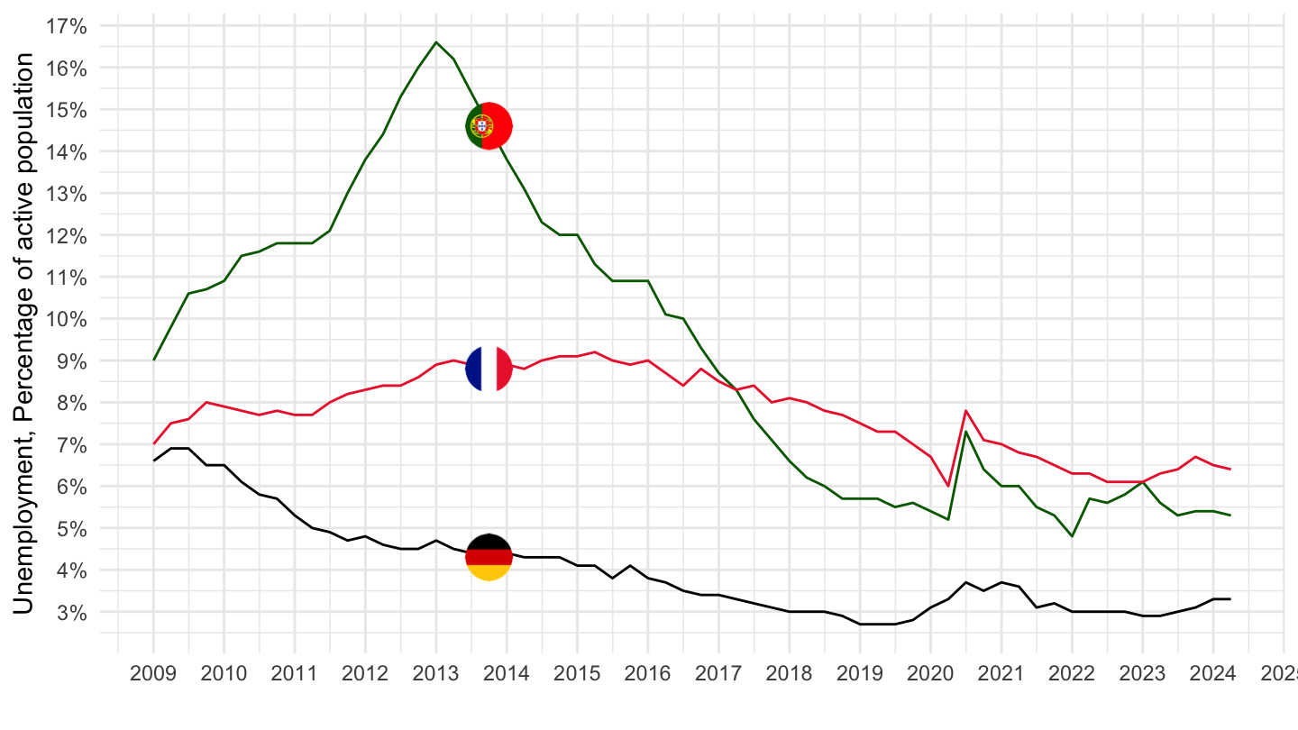
France, Germany, Spain, Netherlands, Italy
All
Code
une_rt_q %>%
  filter(geo %in% c("FR", "DE", "IT", "NL", "ES"),
         age == "Y25-54",
         sex == "T",
         unit == "PC_ACT",
         s_adj == "SA") %>%
  quarter_to_date %>%

  left_join(colors, by = c("Geo" = "country")) %>%
  mutate(values = values/100) %>%
  mutate(color = ifelse(geo == "NL", color2, color)) %>%
  ggplot + geom_line(aes(x = date, y = values, color = color)) +
  theme_minimal() + scale_color_identity() + add_5flags +
  scale_x_date(breaks = as.Date(paste0(seq(1960, 2100, 1), "-01-01")),
               labels = date_format("%Y")) +
  xlab("") + ylab("Unemployment, Percentage of active population") +
  scale_y_continuous(breaks = 0.01*seq(0, 200, 1),
                     labels = scales::percent_format(accuracy = 1))
2009-
Code
une_rt_q %>%
  filter(geo %in% c("FR", "DE", "IT", "NL", "ES"),
         age == "Y25-54",
         sex == "T",
         unit == "PC_ACT",
         s_adj == "SA") %>%
  quarter_to_date %>%
  filter(date >= as.Date("2009-01-01")) %>%

  left_join(colors, by = c("Geo" = "country")) %>%
  mutate(values = values/100) %>%
  mutate(color = ifelse(geo == "NL", color2, color)) %>%
  ggplot + geom_line(aes(x = date, y = values, color = color)) +
  theme_minimal() + scale_color_identity() + add_5flags +
  scale_x_date(breaks = as.Date(paste0(seq(1960, 2100, 1), "-01-01")),
               labels = date_format("%Y")) +
  xlab("") + ylab("Unemployment, Percentage of active population") +
  scale_y_continuous(breaks = 0.01*seq(0, 200, 1),
                     labels = scales::percent_format(accuracy = 1))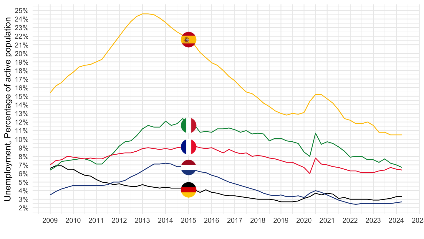
Europe, France, Germany
All
Code
une_rt_q %>%
  filter(geo %in% c("EA20", "FR", "DE"),
         age == "Y25-54",
         sex == "T",
         unit == "PC_ACT",
         s_adj == "SA") %>%
  quarter_to_date %>%

  mutate(Geo = ifelse(geo == "EA20", "Europe", Geo)) %>%
  left_join(colors, by = c("Geo" = "country")) %>%
  mutate(values = values/100) %>%
  mutate(color = ifelse(geo == "FR", color2, color)) %>%
  ggplot + geom_line(aes(x = date, y = values, color = color)) +
  theme_minimal() + scale_color_identity() + add_flags +
  scale_x_date(breaks = as.Date(paste0(seq(1960, 2100, 1), "-01-01")),
               labels = date_format("%Y")) +
  xlab("") + ylab("Unemployment, Percentage of active population") +
  scale_y_continuous(breaks = 0.01*seq(0, 200, 1),
                     labels = scales::percent_format(accuracy = 1))
2009
Code
une_rt_q %>%
  filter(geo %in% c("EA20", "FR", "DE"),
         age == "Y25-54",
         sex == "T",
         unit == "PC_ACT",
         s_adj == "SA") %>%
  quarter_to_date %>%
  filter(date >= as.Date("2009-01-01")) %>%

  mutate(Geo = ifelse(geo == "EA20", "Europe", Geo)) %>%
  left_join(colors, by = c("Geo" = "country")) %>%
  mutate(values = values/100) %>%
  mutate(color = ifelse(geo == "FR", color2, color)) %>%
  ggplot + geom_line(aes(x = date, y = values, color = color)) +
  theme_minimal() + scale_color_identity() + add_flags +
  scale_x_date(breaks = as.Date(paste0(seq(1960, 2100, 1), "-01-01")),
               labels = date_format("%Y")) +
  xlab("") + ylab("Unemployment, Percentage of active population") +
  scale_y_continuous(breaks = 0.01*seq(0, 200, 1),
                     labels = scales::percent_format(accuracy = 1))
Euro Area
Code
une_rt_q %>%
  filter(geo %in% c("EA20"),
         age == "Y20-64",
         sex == "T",
         unit == "PC_ACT",
         s_adj == "SA") %>%
  quarter_to_date %>%
  filter(date >= as.Date("1999-01-01")) %>%

  ggplot + geom_line() + theme_minimal()  +
  aes(x = date, y = values/100) +

  scale_x_date(breaks = as.Date(paste0(seq(1960, 2100, 2), "-01-01")),
               labels = date_format("%Y")) +
  theme(legend.position = c(0.3, 0.25),
        legend.title = element_blank()) +
  xlab("") + ylab("Chômage (en % de la population active)") +
  scale_y_continuous(breaks = 0.01*seq(0, 200, 1),
                     labels = scales::percent_format(accuracy = 1))