GDP per capita in PPS
Data - Eurostat
Info
LAST_DOWNLOAD
Code
tibble(LAST_DOWNLOAD = as.Date(file.info("~/iCloud/website/data/eurostat/tec00114.RData")$mtime)) %>%
print_table_conditional()| LAST_DOWNLOAD |
|---|
| 2026-03-24 |
LAST_COMPILE
| LAST_COMPILE |
|---|
| 2026-07-22 |
Last
Code
tec00114 %>%
  group_by(time) %>%
  summarise(Nobs = n()) %>%
  arrange(desc(time)) %>%
  head(1) %>%
print_table_conditional()| time | Nobs |
|---|---|
| 2024 | 42 |
Info
- Volume indices of real expenditure per capita (in PPS_EU27_2020=100)
indic_ppp
Code
tec00114 %>%
  left_join(indic_ppp, by = "indic_ppp") %>%
  group_by(indic_ppp, Indic_ppp) %>%
  summarise(Nobs = n()) %>%
  arrange(desc(indic_ppp)) %>%
print_table_conditional()| indic_ppp | Indic_ppp | Nobs |
|---|---|---|
| VI_PPS_EU27_2020_HAB | Volume indices of real expenditure per capita (in PPS_EU27_2020=100) | 504 |
time
Code
tec00114 %>%
  group_by(time) %>%
  summarise(Nobs = n()) %>%
  arrange(desc(time)) %>%
print_table_conditional()| time | Nobs |
|---|---|
| 2024 | 42 |
| 2023 | 42 |
| 2022 | 42 |
| 2021 | 42 |
| 2020 | 42 |
| 2019 | 42 |
| 2018 | 42 |
| 2017 | 42 |
| 2016 | 42 |
| 2015 | 42 |
| 2014 | 42 |
| 2013 | 42 |
geo
Code
tec00114 %>%
  left_join(geo, by = "geo") %>%
  group_by(geo, Geo) %>%
  summarise(Nobs = n()) %>%
  arrange(-Nobs) %>%
  mutate(Geo = ifelse(geo == "DE", "Germany", Geo)) %>%
  mutate(Flag = gsub(" ", "-", str_to_lower(Geo)),
         Flag = paste0('<img src="../../icon/flag/vsmall/', Flag, '.png" alt="Flag">')) %>%
  select(Flag, everything()) %>%
  {if (is_html_output()) datatable(., filter = 'top', rownames = F, escape = F) else .}
1995-2024
Code
tec00114 %>%
  filter(time %in% c("1995", "2024")) %>%
  left_join(geo, by = "geo") %>%
  select(time, values, geo, Geo) %>%
  spread(time, values) %>%
  arrange(desc(`2024`)) %>%
  mutate(Geo = ifelse(geo == "DE", "Germany", Geo)) %>%
  mutate(Flag = gsub(" ", "-", str_to_lower(Geo)),
         Flag = paste0('<img src="../../icon/flag/vsmall/', Flag, '.png" alt="Flag">')) %>%
  select(Flag, everything()) %>%
  {if (is_html_output()) datatable(., filter = 'top', rownames = F, escape = F) else .}
Germany, France, Italy
Code
tec00114 %>%
  filter(geo %in% c("FR", "DE", "IT", "ES")) %>%
  select(time, geo, values) %>%
  year_to_date %>%
  left_join(geo, by = "geo") %>%
  left_join(colors, by = c("Geo" = "country")) %>%
  ggplot() + geom_line(aes(x = date, y = values, color = color)) +
  scale_color_identity() + add_4flags +
  theme_minimal()  + xlab("") + ylab("") +
  scale_x_date(breaks = as.Date(paste0(seq(1960,2100, 1), "-01-01")),
               labels = date_format("%Y")) +
  theme(legend.position = c(0.35, 0.85),
        legend.title = element_blank()) +
  scale_y_continuous(breaks = seq(0, 200, 2)) +
  geom_hline(yintercept = 100, linetype = "dashed")
Poland, Hungary, Greece
Code
tec00114 %>%
  filter(geo %in% c("EL", "PL", "HU")) %>%
  select(time, geo, values) %>%
  year_to_date %>%
  left_join(geo, by = "geo") %>%
  left_join(colors, by = c("Geo" = "country")) %>%
  ggplot() + geom_line(aes(x = date, y = values, color = color)) +
  scale_color_identity() + add_3flags +
  theme_minimal()  + xlab("") + ylab("PIB/hab., Parité de Pouvoir d'Achat (EU-27 2020 = 100)") +
  scale_x_date(breaks = as.Date(paste0(seq(1960,2100, 1), "-01-01")),
               labels = date_format("%Y")) +
  theme(legend.position = c(0.35, 0.85),
        legend.title = element_blank()) +
  scale_y_continuous(breaks = seq(0, 200, 2)) +
  geom_hline(yintercept = 100, linetype = "dashed")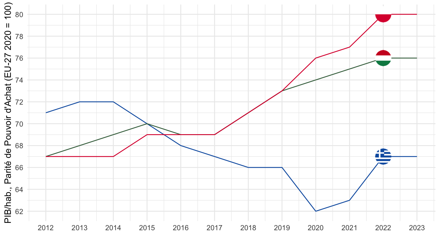
Poland, Hungary, Greece, Germany, France, Italy, Spain, Netherlands
Code
tec00114 %>%
  filter(geo %in% c("EL", "PL", "HU", "FR", "DE", "IT", "ES", "NL")) %>%
  select(time, geo, values) %>%
  year_to_date %>%
  left_join(geo, by = "geo") %>%
  left_join(colors, by = c("Geo" = "country")) %>%
  ggplot() + geom_line(aes(x = date, y = values, color = color)) +
  scale_color_identity() + add_8flags +
  theme_minimal()  + xlab("") + ylab("PIB/hab., Parité de Pouvoir d'Achat (EU-27 2020 = 100)") +
  scale_x_date(breaks = as.Date(paste0(seq(1960,2100, 1), "-01-01")),
               labels = date_format("%Y")) +
  theme(legend.position = c(0.35, 0.85),
        legend.title = element_blank()) +
  scale_y_log10(breaks = seq(0, 200, 5)) +
  geom_hline(yintercept = 100, linetype = "dashed")
Poland, Greece, Germany, France, Italy, Spain
Code
load_data("eurostat/geo_fr.RData")
geo_fr <- geo %>%
  setNames(c("geo", "Geo_fr"))
load_data("eurostat/geo.RData")
tec00114 %>%
  filter(geo %in% c("EL", "PL", "FR", "DE")) %>%
  select(time, geo, values) %>%
  year_to_date %>%
  left_join(geo, by = "geo") %>%
  left_join(geo_fr, by = "geo") %>%
  left_join(colors, by = c("Geo" = "country")) %>%
  ggplot() + geom_line(aes(x = date, y = values, color = color)) +
  scale_color_identity() + add_flags +
  theme_minimal()  + xlab("") + ylab("PIB/hab., Parité de Pouvoir d'Achat (EU-27 2020 = 100)") +
  scale_x_date(breaks = as.Date(paste0(seq(1960,2100, 1), "-01-01")),
               labels = date_format("%Y")) +
  theme(legend.position = c(0.35, 0.85),
        legend.title = element_blank()) +
  scale_y_log10(breaks = seq(0, 200, 5)) +
  geom_hline(yintercept = 100, linetype = "dashed") +
  geom_text(data = . %>% filter(date == max(date)), aes(x = date, y = values, label = Geo_fr, color = color))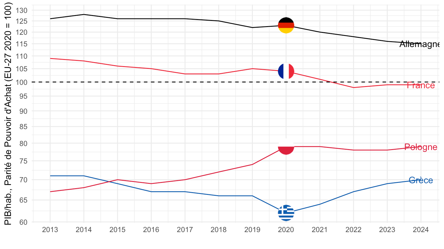
Poland, Greece, Germany, France, Italy, Spain
Code
load_data("eurostat/geo_fr.RData")
geo_fr <- geo %>%
  setNames(c("geo", "Geo_fr"))
load_data("eurostat/geo.RData")
tec00114 %>%
  filter(geo %in% c("EL", "PL", "FR", "DE", "IT", "ES")) %>%
  select(time, geo, values) %>%
  year_to_date %>%
  left_join(geo, by = "geo") %>%
  left_join(geo_fr, by = "geo") %>%
  left_join(colors, by = c("Geo" = "country")) %>%
  ggplot() + geom_line(aes(x = date, y = values, color = color)) +
  scale_color_identity() + add_6flags +
  theme_minimal()  + xlab("") + ylab("PIB/hab., Parité de Pouvoir d'Achat (EU-27 2020 = 100)") +
  scale_x_date(breaks = as.Date(paste0(seq(1960,2100, 1), "-01-01")),
               labels = date_format("%Y")) +
  theme(legend.position = c(0.35, 0.85),
        legend.title = element_blank()) +
  scale_y_log10(breaks = seq(0, 200, 5)) +
  geom_hline(yintercept = 100, linetype = "dashed") +
  geom_text(data = . %>% filter(date == max(date)), aes(x = date, y = values, label = Geo_fr, color = color))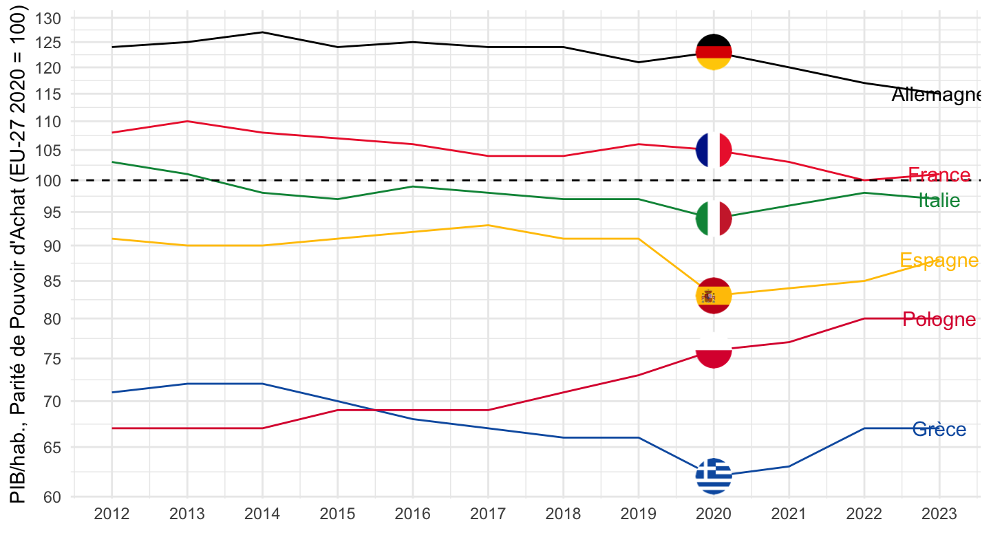
Poland, Hungary, Greece, Germany, France, Italy, Spain, United States
Code
tec00114 %>%
  filter(geo %in% c("FR", "DE", "IT", "ES", "US", "EU27_2020", "UK", "NL")) %>%
  select(time, geo, values) %>%
  year_to_date %>%
  left_join(geo, by = "geo") %>%
  mutate(Geo = ifelse(geo == "EU27_2020", "Europe", Geo)) %>%
  left_join(colors, by = c("Geo" = "country")) %>%
  mutate(color = ifelse(geo == "UK", color2, color)) %>%
  ggplot() + geom_line(aes(x = date, y = values, color = color)) +
  scale_color_identity() + add_8flags +
  theme_minimal()  + xlab("") + ylab("PIB/hab., Parité de Pouvoir d'Achat (EU-27 2020 = 100)") +
  scale_x_date(breaks = as.Date(paste0(seq(1960,2100, 1), "-01-01")),
               labels = date_format("%Y")) +
  theme(legend.position = c(0.35, 0.85),
        legend.title = element_blank()) +
  scale_y_log10(breaks = seq(0, 200, 5)) +
  geom_hline(yintercept = 100, linetype = "dashed")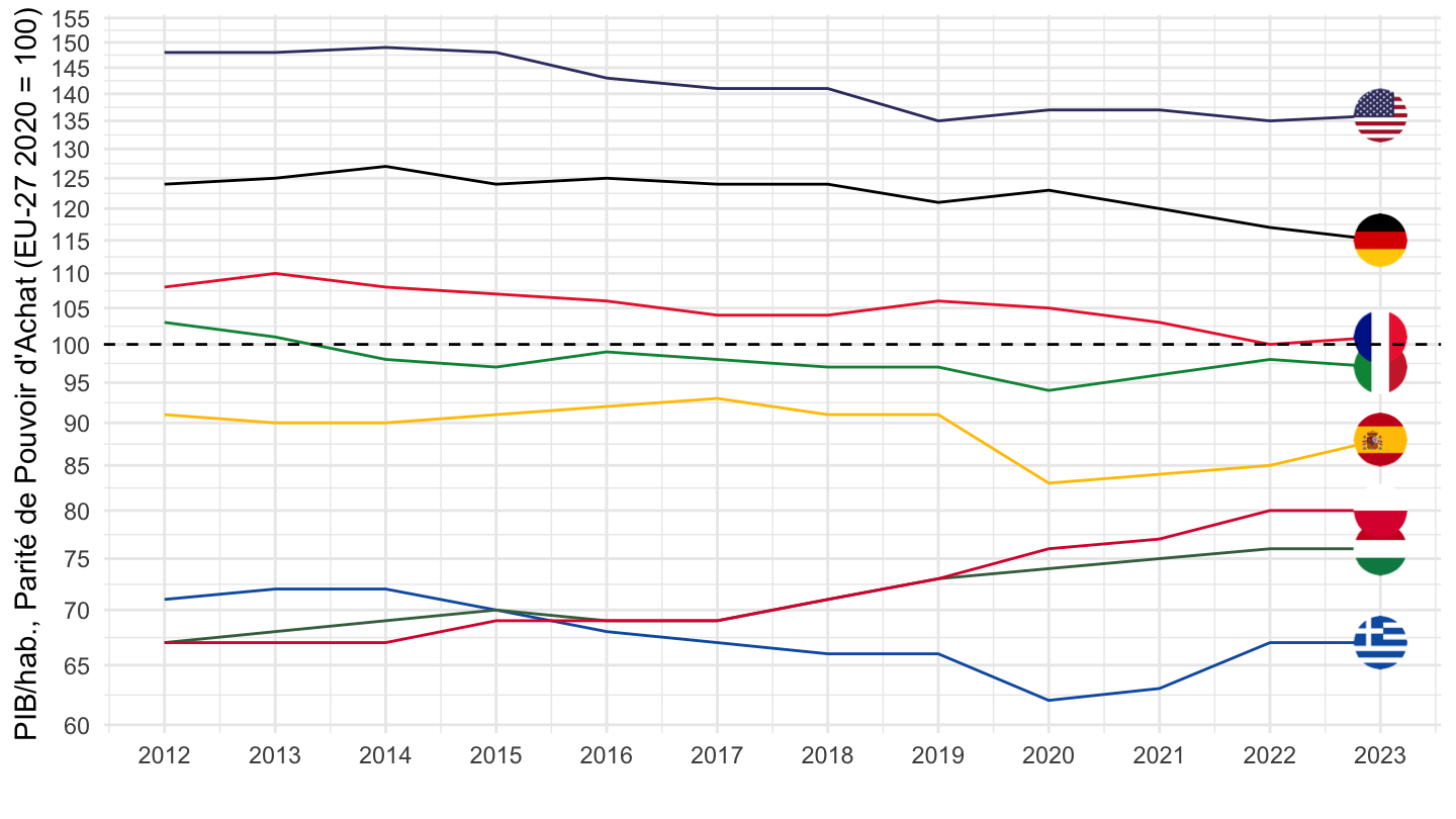
Poland, Hungary, Greece, Germany, France, Italy, Spain, United States
Code
tec00114 %>%
  filter(geo %in% c("EL", "PL", "HU", "FR", "DE", "IT", "ES", "US", "UK")) %>%
  select(time, geo, values) %>%
  year_to_date %>%
  left_join(geo, by = "geo") %>%
  left_join(colors, by = c("Geo" = "country")) %>%
  mutate(color = ifelse(geo == "UK", color2, color)) %>%
  ggplot() + geom_line(aes(x = date, y = values, color = color)) +
  scale_color_identity() + add_flags +
  theme_minimal()  + xlab("") + ylab("PIB/hab., Parité de Pouvoir d'Achat\nEU-27 2020 = 100") +
  scale_x_date(breaks = as.Date(paste0(seq(1960,2100, 1), "-01-01")),
               labels = date_format("%Y")) +
  theme(legend.position = c(0.35, 0.85),
        legend.title = element_blank()) +
  scale_y_log10(breaks = seq(0, 200, 5)) +
  geom_hline(yintercept = 100, linetype = "dashed")
Germany, France, Italy, United States, Switzerland, United Kingdom
Code
tec00114 %>%
  filter(geo %in% c("FR", "DE", "IT", "UK", "CH", "US")) %>%
  select(time, geo, values) %>%
  year_to_date %>%
  left_join(geo, by = "geo") %>%
  left_join(colors, by = c("Geo" = "country")) %>%
  ggplot() + geom_line(aes(x = date, y = values, color = color)) +
  scale_color_identity() + add_6flags +
  theme_minimal()  + xlab("") + ylab("PIB/hab., Parité de Pouvoir d'Achat (EU-27 2020 = 100)") +
  scale_x_date(breaks = as.Date(paste0(seq(1960,2100, 1), "-01-01")),
               labels = date_format("%Y")) +
  theme(legend.position = c(0.35, 0.85),
        legend.title = element_blank()) +
  scale_y_log10(breaks = seq(0, 200, 5)) +
  geom_hline(yintercept = 100, linetype = "dashed")