| source | dataset | Title | .html | .rData |
|---|---|---|---|---|
| eurostat | prc_hicp_ctrb | Contributions to euro area annual inflation (in percentage points) | 2026-06-04 | 2026-04-26 |
Gross domestic product (GDP) at current market prices by NUTS 2 regions
Data - Eurostat
Info
LAST_DOWNLOAD
Code
tibble(LAST_DOWNLOAD = as.Date(file.info("~/iCloud/website/data/eurostat/nama_10r_2gdp.RData")$mtime)) %>%
print_table_conditional()| LAST_DOWNLOAD |
|---|
| 2026-04-14 |
LAST_COMPILE
| LAST_COMPILE |
|---|
| 2026-06-21 |
Last
Code
nama_10r_2gdp %>%
  group_by(time) %>%
  summarise(Nobs = n()) %>%
  arrange(desc(time)) %>%
  head(1) %>%
print_table_conditional()| time | Nobs |
|---|---|
| 2024 | 3002 |
unit
Code
nama_10r_2gdp %>%
  left_join(unit, by = "unit") %>%
  group_by(unit, Unit) %>%
  summarise(Nobs = n()) %>%
  arrange(-Nobs) %>%
print_table_conditional()| unit | Unit | Nobs |
|---|---|---|
| MIO_EUR | Million euro | 11453 |
| MIO_NAC | Million units of national currency | 11453 |
| MIO_PPS_EU27_2020 | Million purchasing power standards (PPS, EU27 from 2020) | 11453 |
| EUR_HAB | Euro per inhabitant | 10393 |
| EUR_HAB_EU27_2020 | Euro per inhabitant in percentage of the EU27 (from 2020) average | 10393 |
| PPS_EU27_2020_HAB | Purchasing power standard (PPS, EU27 from 2020), per inhabitant | 10393 |
| PPS_HAB_EU27_2020 | Purchasing power standard (PPS, EU27 from 2020), per inhabitant in percentage of the EU27 (from 2020) average | 10393 |
geo
Code
nama_10r_2gdp %>%
  left_join(geo, by = "geo") %>%
  group_by(geo, Geo) %>%
  summarise(Nobs = n()) %>%
  arrange(-Nobs) %>%
  {if (is_html_output()) datatable(., filter = 'top', rownames = F) else .}
time
Code
nama_10r_2gdp %>%
  group_by(time) %>%
  summarise(Nobs = n()) %>%
  arrange(desc(time)) %>%
print_table_conditional()| time | Nobs |
|---|---|
| 2024 | 3002 |
| 2023 | 3017 |
| 2022 | 3064 |
| 2021 | 3129 |
| 2020 | 3129 |
| 2019 | 3129 |
| 2018 | 3129 |
| 2017 | 3129 |
| 2016 | 3129 |
| 2015 | 3129 |
| 2014 | 3129 |
| 2013 | 3125 |
| 2012 | 3125 |
| 2011 | 3077 |
| 2010 | 3077 |
| 2009 | 3077 |
| 2008 | 3077 |
| 2007 | 2950 |
| 2006 | 2950 |
| 2005 | 2929 |
| 2004 | 2929 |
| 2003 | 2929 |
| 2002 | 2825 |
| 2001 | 2873 |
| 2000 | 2873 |
France
Table
Code
nama_10r_2gdp %>%
  filter(grepl("FR", geo),
         unit %in% c("EUR_HAB", "PPS_EU27_2020_HAB"),
         time == "2020") %>%
  left_join(geo, by = "geo") %>%
  spread(unit, values) %>%
  mutate(pps = PPS_EU27_2020_HAB/EUR_HAB) %>%
  select(-time) %>%
  arrange(-pps) %>%
  print_table_conditional
Ile de France
Code
nama_10r_2gdp %>%
  filter(unit %in% c("EUR_HAB", "PPS_EU27_2020_HAB"),
         geo %in% c("FRC2", "FR10", "FRG0", "FRD1")) %>%
  left_join(geo, by = "geo") %>%
  spread(unit, values) %>%
  mutate(values = PPS_EU27_2020_HAB/EUR_HAB) %>%
  year_to_date %>%
  ggplot + geom_line(aes(x = date, y = values, color = Geo)) +
  theme_minimal() + xlab("") + ylab("PPS") +
  theme(legend.title = element_blank(),
        legend.position = c(0.75, 0.85)) +
  scale_x_date(breaks = seq(1960, 2026, 5) %>% paste0("-01-01") %>% as.Date,
               labels = date_format("%Y")) +
  scale_y_continuous(breaks = 0.01*seq(-500, 200, 1),
                     labels = percent_format(accuracy = 1))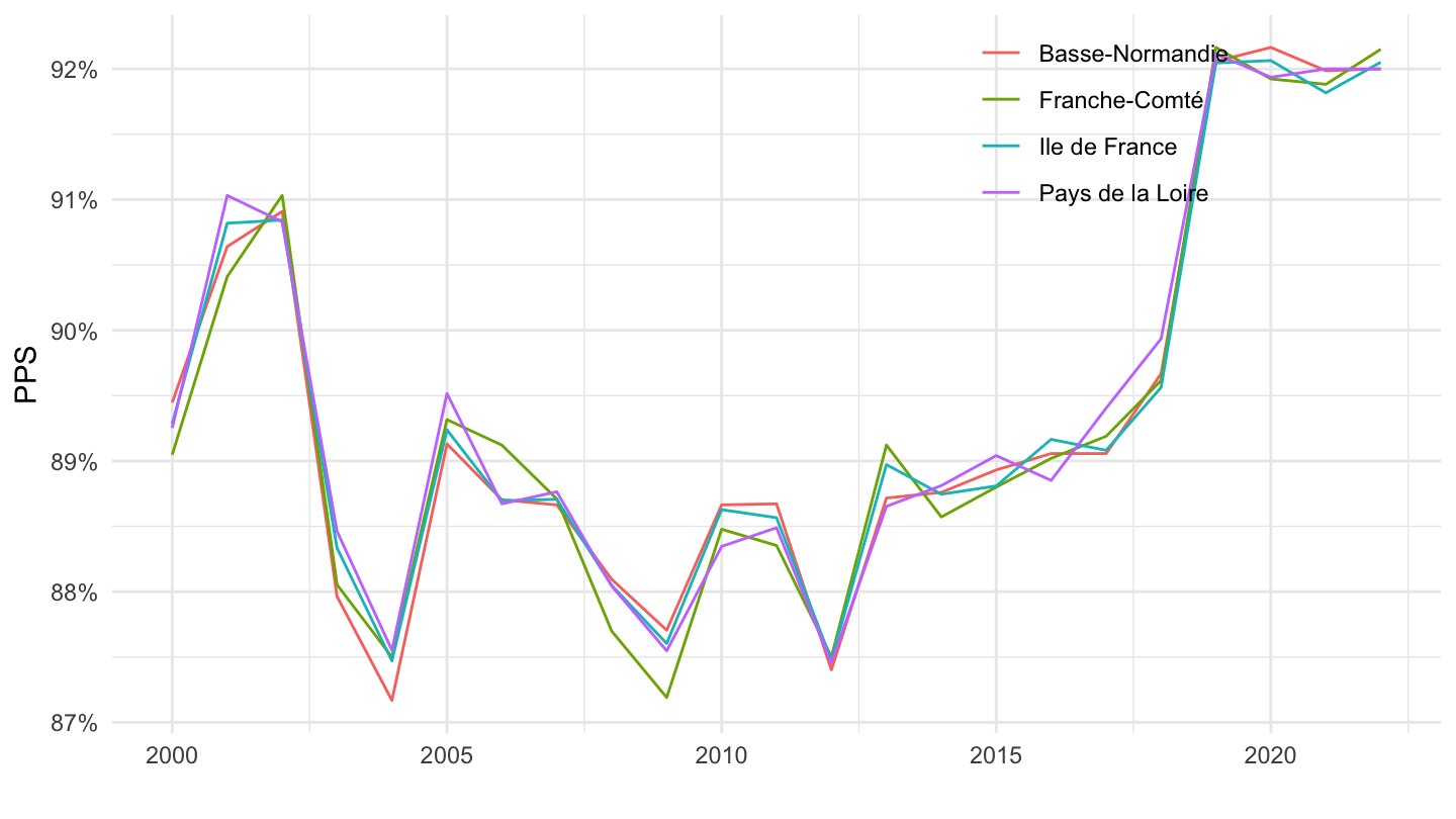
Germany
Table
Code
nama_10r_2gdp %>%
  filter(grepl("DE", geo),
         unit %in% c("EUR_HAB", "PPS_EU27_2020_HAB"),
         time == "2020") %>%
  left_join(geo, by = "geo") %>%
  spread(unit, values) %>%
  mutate(pps = PPS_EU27_2020_HAB/EUR_HAB) %>%
  select(-time) %>%
  arrange(-pps) %>%
  print_table_conditional
Régions
Code
nama_10r_2gdp %>%
  filter(unit %in% c("EUR_HAB", "PPS_EU27_2020_HAB"),
         geo %in% c("DEB3", "DEE0", "DE40", "DE13")) %>%
  left_join(geo, by = "geo") %>%
  spread(unit, values) %>%
  mutate(values = PPS_EU27_2020_HAB/EUR_HAB) %>%
  year_to_date %>%
  ggplot + geom_line(aes(x = date, y = values, color = Geo)) +
  theme_minimal() + xlab("") + ylab("PPS") +
  theme(legend.title = element_blank(),
        legend.position = c(0.75, 0.15)) +
  scale_x_date(breaks = seq(1960, 2026, 2) %>% paste0("-01-01") %>% as.Date,
               labels = date_format("%Y")) +
  scale_y_continuous(breaks = 0.01*seq(-500, 200, 1),
                     labels = percent_format(accuracy = 1))
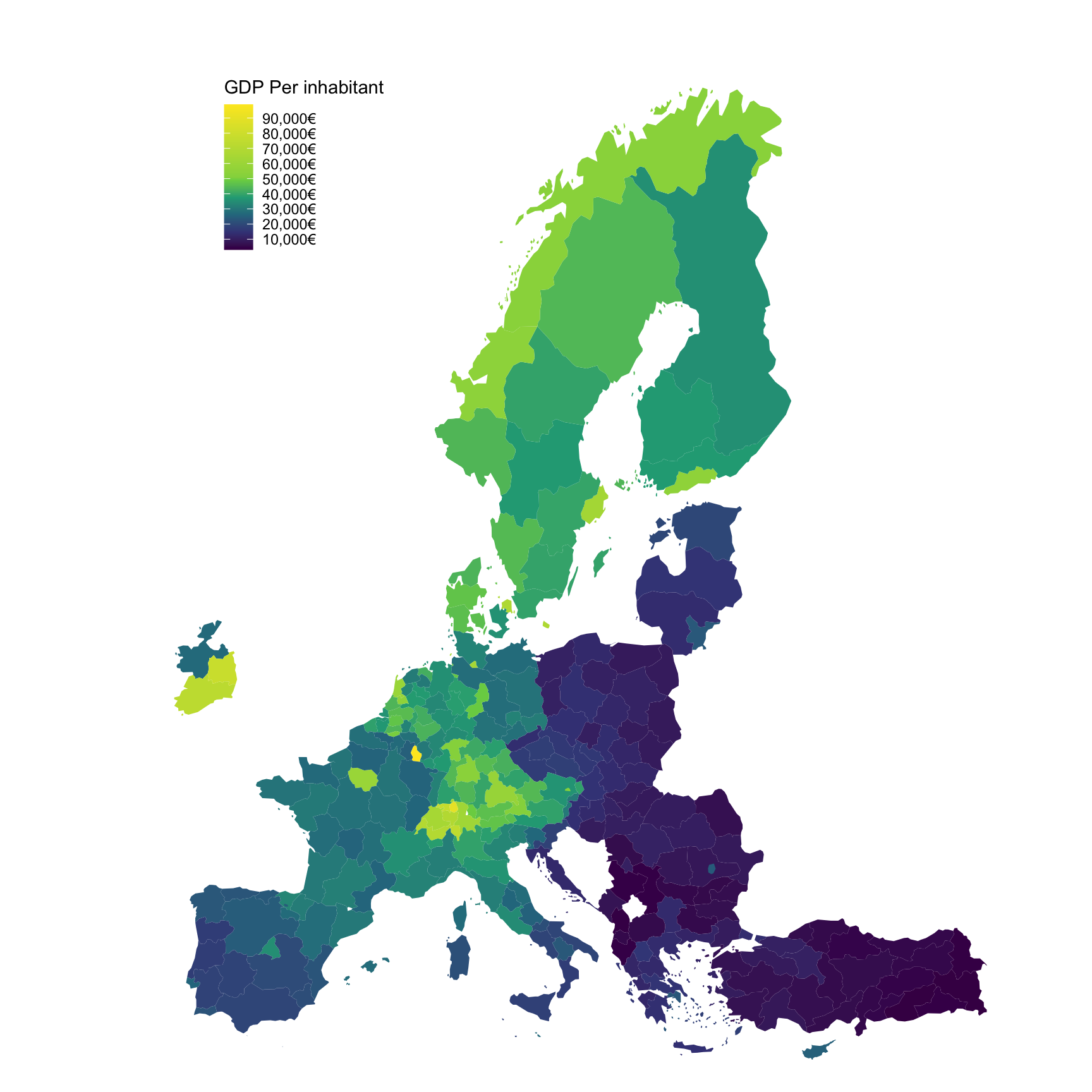
Maps
2019
Code
nama_10r_2gdp %>%
  filter(time == "2019",
         unit == "EUR_HAB") %>%
  left_join(geo, by = "geo") %>%
  select(geo, Geo, values) %>%
  right_join(europe_NUTS2, by = "geo") %>%
  filter(long >= -15, lat >= 33) %>%
  ggplot(., aes(x = long, y = lat, group = group, fill = values)) +
  geom_polygon() + coord_map() +
  scale_fill_viridis_c(na.value = "white",
                       labels = scales::dollar_format(accuracy = 1, prefix = "", suffix = "€"),
                       breaks = seq(10000, 120000, 10000),
                       values = c(0, 0.1, 0.2, 0.3, 0.4, 0.5, 1)) +
  theme_void() + theme(legend.position = c(0.25, 0.85)) +
  labs(fill = "GDP Per inhabitant")
2018
Code
nama_10r_2gdp %>%
  filter(time == "2018",
         unit == "EUR_HAB") %>%
  left_join(geo, by = "geo") %>%
  select(geo, Geo, values) %>%
  right_join(europe_NUTS2, by = "geo") %>%
  filter(long >= -15, lat >= 33) %>%
  ggplot(., aes(x = long, y = lat, group = group, fill = values)) +
  geom_polygon() + coord_map() +
  scale_fill_viridis_c(na.value = "white",
                       labels = scales::dollar_format(accuracy = 1, prefix = "", suffix = "€"),
                       breaks = seq(10000, 120000, 10000),
                       values = c(0, 0.1, 0.2, 0.3, 0.4, 0.5, 1)) +
  theme_void() + theme(legend.position = c(0.25, 0.85)) +
  labs(fill = "GDP Per inhabitant")