Employment rates by sex, age and educational attainment level (%) - lfsq_ergaed
Data - Eurostat
Info
Last observation: Quarterly: 2026Q1 (N = 19,804)
First observation: Quarterly: 1998Q1 (N = 3,114)
Last data update: 23 jul 2026, 22:46. Last compile: 24 jul 2026, 02:18
Structure
isced11
Code
load_data("eurostat/isced11_fr.RData")
lfsq_ergaed %>%

  group_by(isced11, Isced11) %>%
  summarise(Nobs = n()) %>%
  arrange(-Nobs) %>%
print_table_conditional()| isced11 | Isced11 | Nobs |
|---|---|---|
| TOTAL | All ISCED 2011 levels | 332730 |
| ED0-2 | Less than primary, primary and lower secondary education (levels 0-2) | 331190 |
| ED3_4 | Upper secondary and post-secondary non-tertiary education (levels 3 and 4) | 331174 |
| ED5-8 | Tertiary education (levels 5-8) | 324764 |
| NRP | No response | 115086 |
| ED35_45 | Upper secondary and post-secondary non-tertiary education - vocational (levels 35 and 45) | 82842 |
| ED34_44 | Upper secondary and post-secondary non-tertiary education - general (levels 34 and 44) | 81890 |
| NAP | Not applicable | 132 |
France, EU, Italy, Germany, Spain, Netherlands
Peu d’éducation
Y15-39
Code
lfsq_ergaed %>%
  filter(isced11 == "ED0-2",
         age == "Y15-39",
         geo %in% c("EA20", "DE", "ES", "FR", "IT"),
         sex == "T") %>%
  quarter_to_date() %>%
  filter(date >= as.Date("1995-01-01")) %>%

  mutate(Geo = ifelse(geo == "DE", "Germany", Geo)) %>%
  mutate(Geo = ifelse(geo == "EA20", "Europe", Geo)) %>%
  left_join(colors, by = c("Geo" = "country")) %>%
  mutate(color = ifelse(geo == "EA20", color2, color)) %>%
  mutate(color = ifelse(geo == "ES", color2, color)) %>%
  mutate(values = values / 100) %>%
  ggplot(.) + geom_line(aes(x = date, y = values, color = color)) +
  theme_minimal() + xlab("") + ylab("Taux d'emploi (1er cycle de l'enseignement secondaire)") +
  scale_color_identity() + add_5flags +
  scale_x_date(breaks = seq(1960, 2100, 5) %>% paste0("-01-01") %>% as.Date,
               labels = date_format("%Y")) +
  scale_y_continuous(breaks = 0.01*seq(-500, 200, 2),
                     labels = percent_format(accuracy = 1))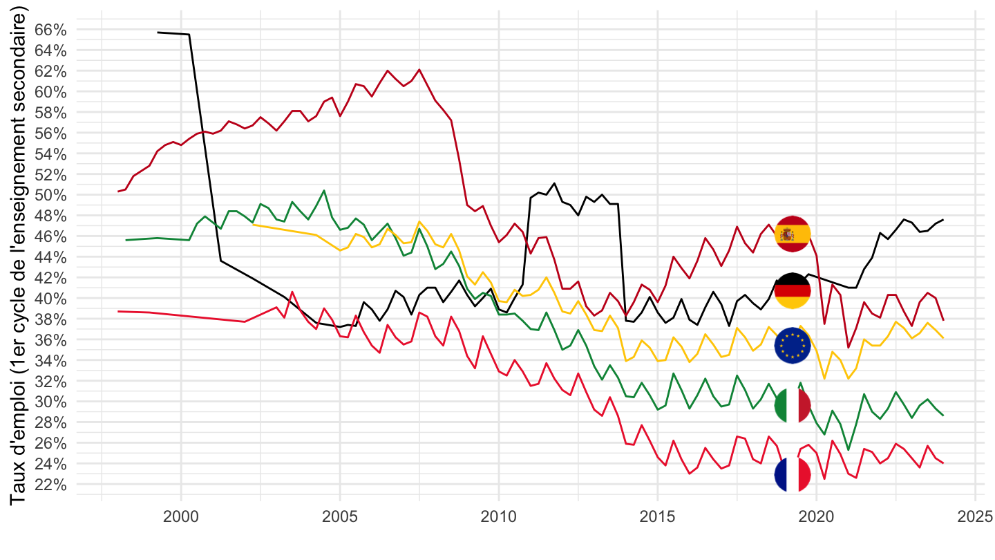
Y40-64
Code
lfsq_ergaed %>%
  filter(isced11 == "ED0-2",
         age == "Y40-64",
         geo %in% c("EA20", "DE", "ES", "FR", "IT"),
         sex == "T") %>%
  quarter_to_date() %>%
  filter(date >= as.Date("2005-01-01")) %>%

  mutate(Geo = ifelse(geo == "DE", "Germany", Geo)) %>%
  mutate(Geo = ifelse(geo == "EA20", "Europe", Geo)) %>%
  left_join(colors, by = c("Geo" = "country")) %>%
  mutate(color = ifelse(geo == "EA20", color2, color)) %>%
  mutate(color = ifelse(geo == "ES", color2, color)) %>%
  mutate(values = values / 100) %>%
  ggplot(.) + geom_line(aes(x = date, y = values, color = color)) +
  theme_minimal() + xlab("") + ylab("Taux d'emploi 40-64 (1er cycle du secondaire)") +
  scale_color_identity() + add_5flags +
  scale_x_date(breaks = seq(1960, 2100, 5) %>% paste0("-01-01") %>% as.Date,
               labels = date_format("%Y")) +
  scale_y_continuous(breaks = 0.01*seq(-500, 200, 2),
                     labels = percent_format(accuracy = 1))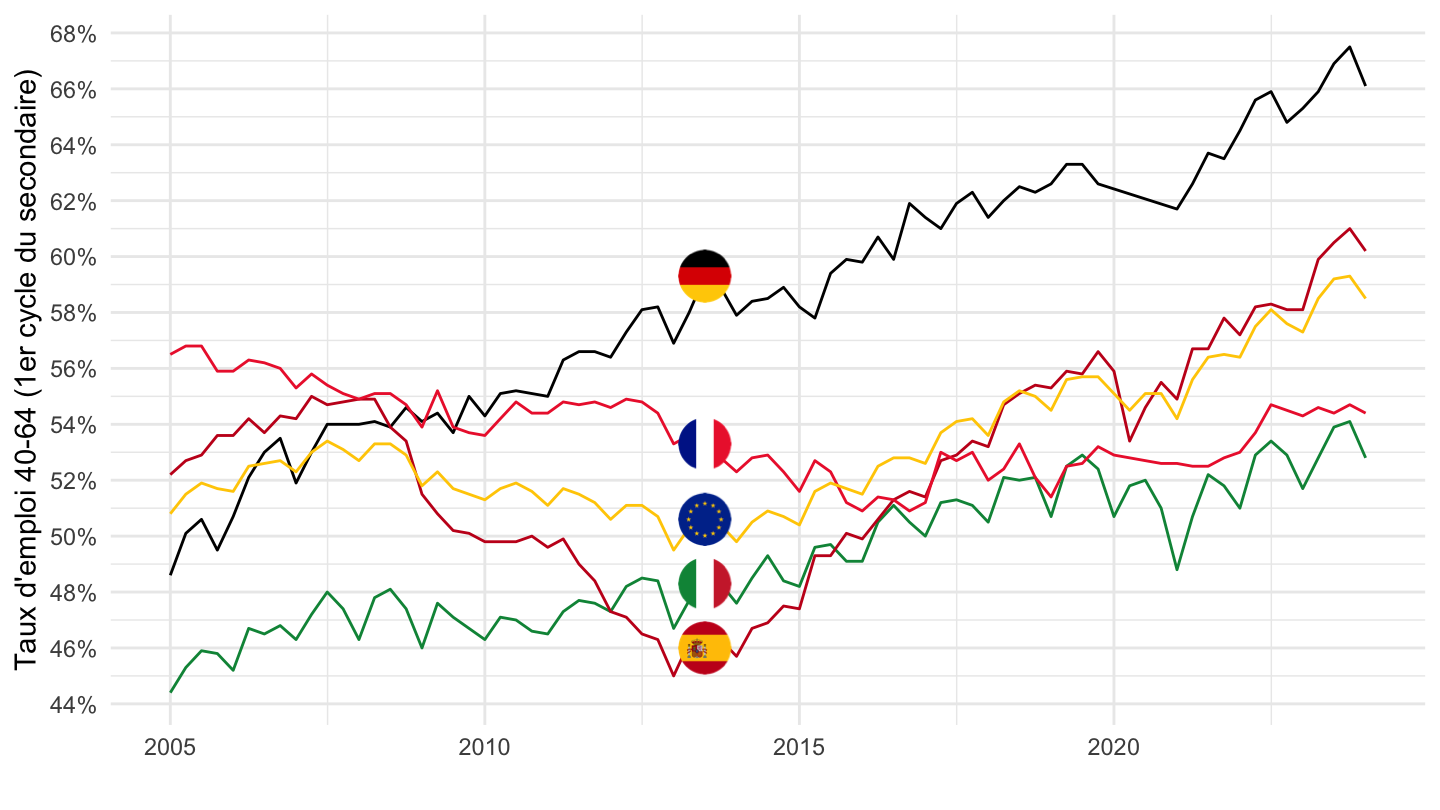
Males
Code
lfsq_ergaed %>%
  filter(isced11 == "ED0-2",
         age == "Y40-64",
         geo %in% c("EA20", "DE", "ES", "FR", "IT"),
         sex == "M") %>%
  quarter_to_date() %>%
  filter(date >= as.Date("2005-01-01")) %>%

  mutate(Geo = ifelse(geo == "DE", "Germany", Geo)) %>%
  mutate(Geo = ifelse(geo == "EA20", "Europe", Geo)) %>%
  left_join(colors, by = c("Geo" = "country")) %>%
  mutate(color = ifelse(geo == "EA20", color2, color)) %>%
  mutate(color = ifelse(geo == "ES", color2, color)) %>%
  mutate(values = values / 100) %>%
  ggplot(.) + geom_line(aes(x = date, y = values, color = color)) +
  theme_minimal() + xlab("") + ylab("Taux d'emploi M 40-64 (1er cycle du secondaire)") +
  scale_color_identity() + add_5flags +
  scale_x_date(breaks = seq(1960, 2100, 5) %>% paste0("-01-01") %>% as.Date,
               labels = date_format("%Y")) +
  scale_y_continuous(breaks = 0.01*seq(-500, 200, 2),
                     labels = percent_format(accuracy = 1))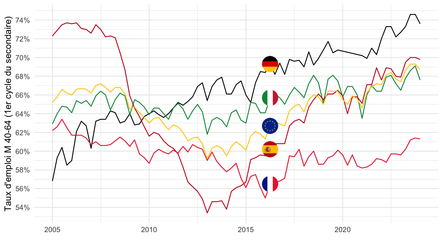
Females
Code
lfsq_ergaed %>%
  filter(isced11 == "ED0-2",
         age == "Y40-64",
         geo %in% c("EA20", "DE", "ES", "FR", "IT"),
         sex == "F") %>%
  quarter_to_date() %>%
  filter(date >= as.Date("2005-01-01")) %>%

  mutate(Geo = ifelse(geo == "DE", "Germany", Geo)) %>%
  mutate(Geo = ifelse(geo == "EA20", "Europe", Geo)) %>%
  left_join(colors, by = c("Geo" = "country")) %>%
  mutate(color = ifelse(geo == "EA20", color2, color)) %>%
  mutate(color = ifelse(geo == "ES", color2, color)) %>%
  mutate(values = values / 100) %>%
  ggplot(.) + geom_line(aes(x = date, y = values, color = color)) +
  theme_minimal() + xlab("") + ylab("Taux d'emploi F 40-64 (1er cycle du secondaire)") +
  scale_color_identity() + add_5flags +
  scale_x_date(breaks = seq(1960, 2100, 5) %>% paste0("-01-01") %>% as.Date,
               labels = date_format("%Y")) +
  scale_y_continuous(breaks = 0.01*seq(-500, 200, 2),
                     labels = percent_format(accuracy = 1))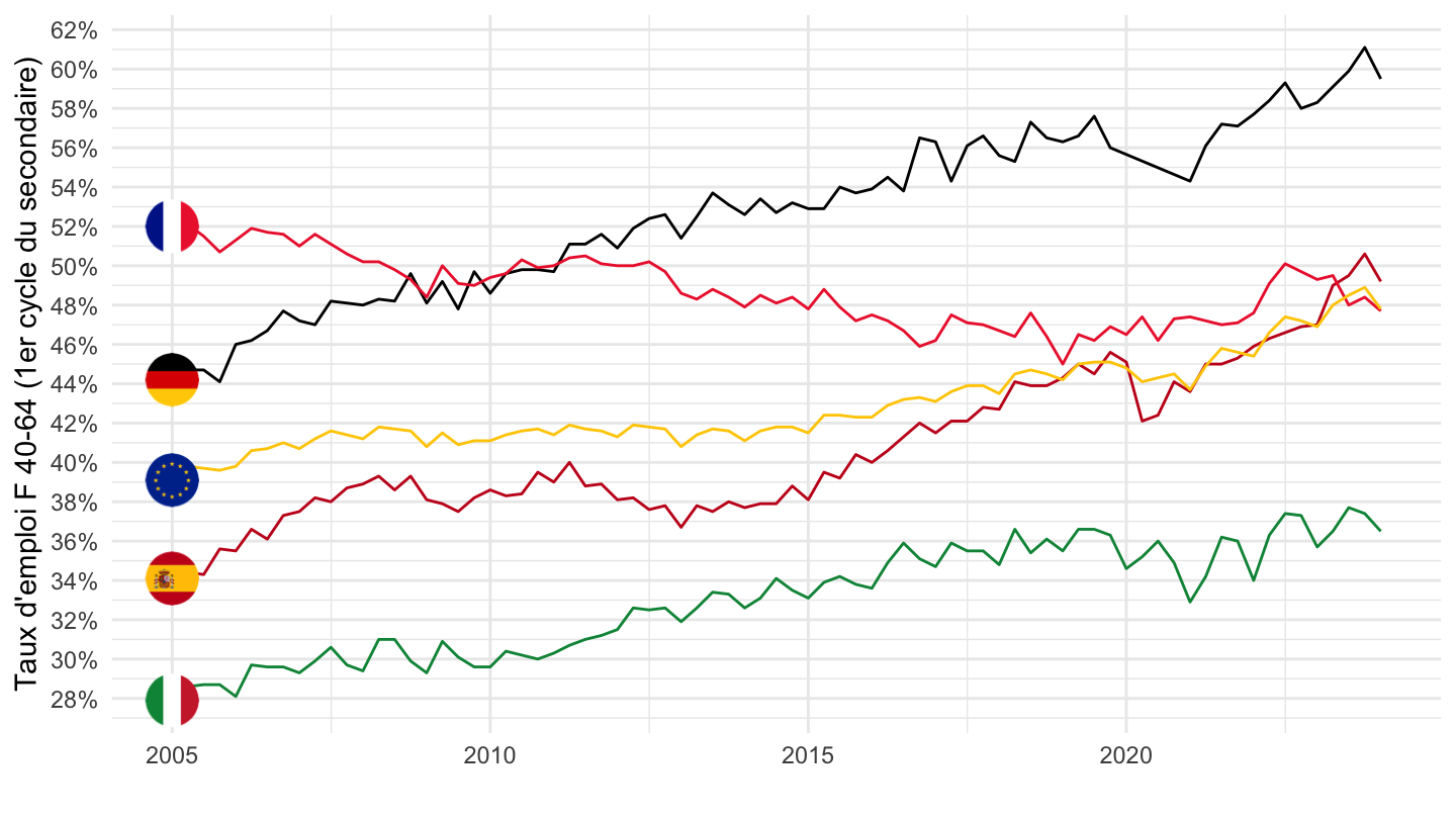
Y15-64
Tous
1995-
Code
lfsq_ergaed %>%
  filter(isced11 == "ED0-2",
         age == "Y15-64",
         geo %in% c("EA20", "DE", "ES", "FR", "IT"),
         sex == "T") %>%
  quarter_to_date() %>%
  filter(date >= as.Date("1995-01-01")) %>%

  mutate(Geo = ifelse(geo == "DE", "Germany", Geo)) %>%
  mutate(Geo = ifelse(geo == "EA20", "Europe", Geo)) %>%
  left_join(colors, by = c("Geo" = "country")) %>%
  mutate(color = ifelse(geo == "EA20", color2, color)) %>%
  mutate(color = ifelse(geo == "ES", color2, color)) %>%
  mutate(values = values / 100) %>%
  ggplot(.) + geom_line(aes(x = date, y = values, color = color)) +
  theme_minimal() + xlab("") + ylab("Taux d'emploi (1er cycle de l'enseignement secondaire)") +
  scale_color_identity() + add_5flags +
  scale_x_date(breaks = seq(1960, 2100, 5) %>% paste0("-01-01") %>% as.Date,
               labels = date_format("%Y")) +
  scale_y_continuous(breaks = 0.01*seq(-500, 200, 2),
                     labels = percent_format(accuracy = 1))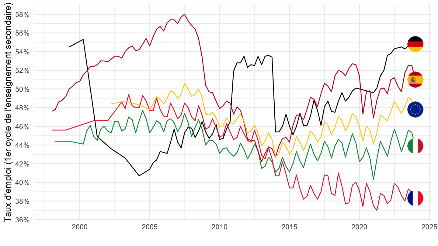
2005-
Code
lfsq_ergaed %>%
  filter(isced11 == "ED0-2",
         age == "Y15-64",
         geo %in% c("EA20", "DE", "ES", "FR", "IT"),
         sex == "T") %>%
  quarter_to_date() %>%
  filter(date >= as.Date("2005-01-01")) %>%

  mutate(Geo = ifelse(geo == "DE", "Germany", Geo)) %>%
  mutate(Geo = ifelse(geo == "EA20", "Europe", Geo)) %>%
  left_join(colors, by = c("Geo" = "country")) %>%
  mutate(color = ifelse(geo == "EA20", color2, color)) %>%
  mutate(color = ifelse(geo == "ES", color2, color)) %>%
  mutate(values = values / 100) %>%
  ggplot(.) + geom_line(aes(x = date, y = values, color = color)) +
  theme_minimal() + xlab("") + ylab("Taux d'emploi (1er cycle du secondaire)") +
  scale_color_identity() + add_5flags +
  scale_x_date(breaks = seq(1960, 2100, 5) %>% paste0("-01-01") %>% as.Date,
               labels = date_format("%Y")) +
  scale_y_continuous(breaks = 0.01*seq(-500, 200, 2),
                     labels = percent_format(accuracy = 1))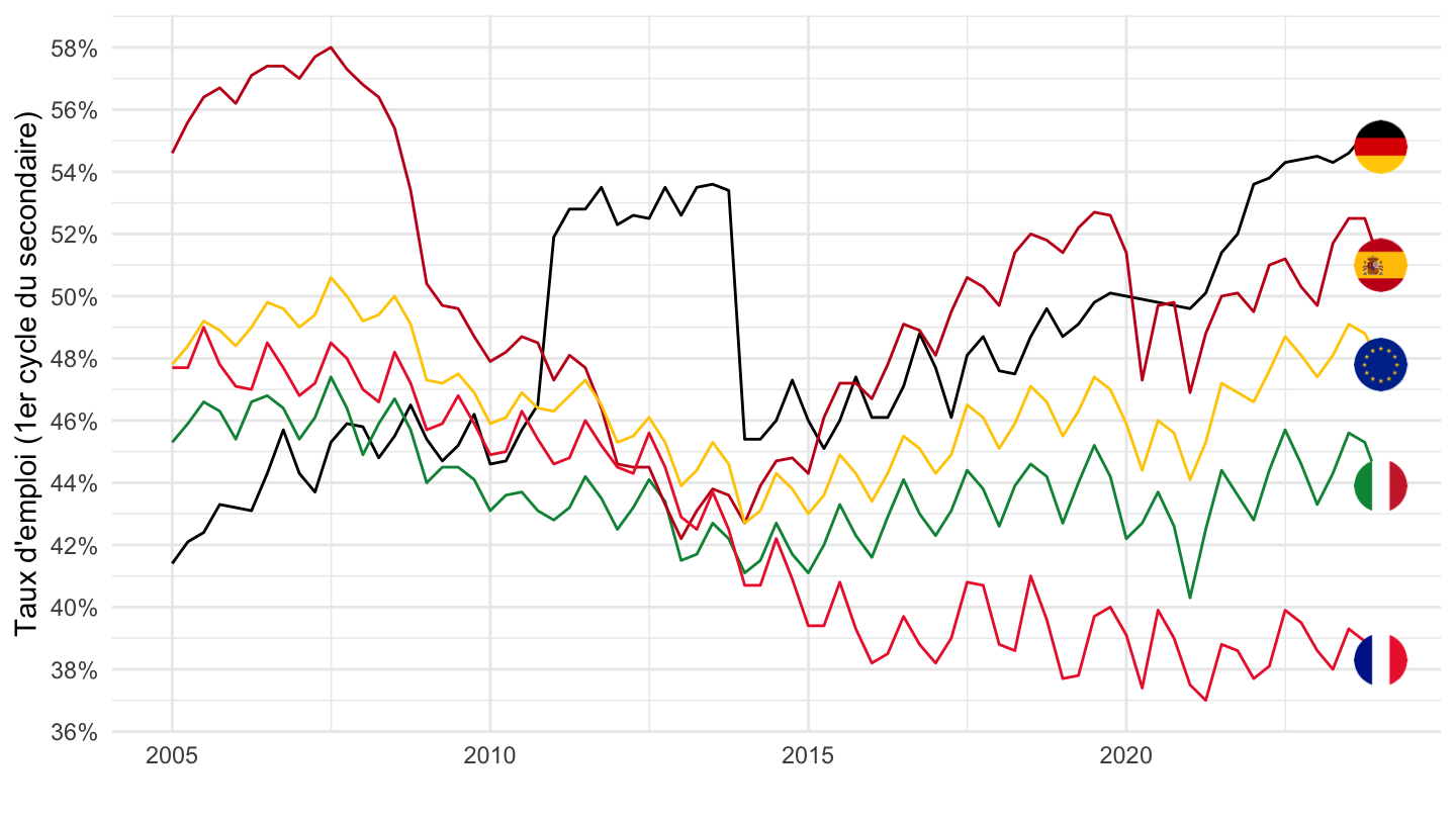
Femmes
Code
lfsq_ergaed %>%
  filter(isced11 == "ED0-2",
         age == "Y15-64",
         geo %in% c("EA20", "DE", "ES", "FR", "IT"),
         sex == "F") %>%
  quarter_to_date() %>%
  filter(date >= as.Date("1995-01-01")) %>%

  mutate(Geo = ifelse(geo == "DE", "Germany", Geo)) %>%
  mutate(Geo = ifelse(geo == "EA20", "Europe", Geo)) %>%
  left_join(colors, by = c("Geo" = "country")) %>%
  mutate(color = ifelse(geo == "EA20", color2, color)) %>%
  mutate(color = ifelse(geo == "ES", color2, color)) %>%
  mutate(values = values / 100) %>%
  ggplot(.) + geom_line(aes(x = date, y = values, color = color)) +
  theme_minimal() + xlab("") + ylab("Taux d'emploi (1er cycle de l'enseignement secondaire)") +
  scale_color_identity() + add_5flags +
  scale_x_date(breaks = seq(1960, 2100, 5) %>% paste0("-01-01") %>% as.Date,
               labels = date_format("%Y")) +
  scale_y_continuous(breaks = 0.01*seq(-500, 200, 2),
                     labels = percent_format(accuracy = 1))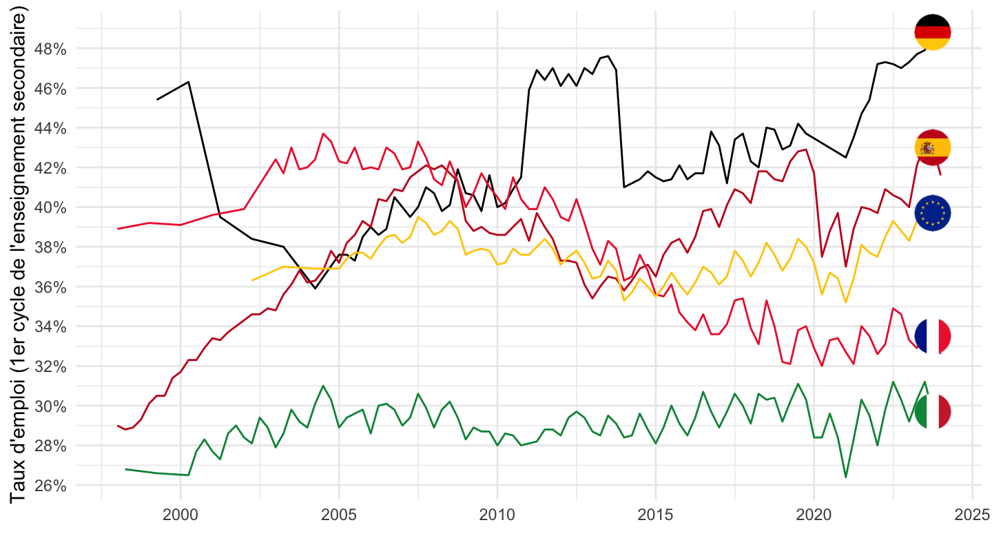
Hommes
Code
lfsq_ergaed %>%
  filter(isced11 == "ED0-2",
         age == "Y15-64",
         geo %in% c("EA20", "DE", "ES", "FR", "IT"),
         sex == "M") %>%
  quarter_to_date() %>%
  filter(date >= as.Date("1995-01-01")) %>%

  mutate(Geo = ifelse(geo == "DE", "Germany", Geo)) %>%
  mutate(Geo = ifelse(geo == "EA20", "Europe", Geo)) %>%
  left_join(colors, by = c("Geo" = "country")) %>%
  mutate(color = ifelse(geo == "EA20", color2, color)) %>%
  mutate(color = ifelse(geo == "ES", color2, color)) %>%
  mutate(values = values / 100) %>%
  ggplot(.) + geom_line(aes(x = date, y = values, color = color)) +
  theme_minimal() + xlab("") + ylab("Taux d'emploi (1er cycle de l'enseignement secondaire)") +
  scale_color_identity() + add_5flags +
  scale_x_date(breaks = seq(1960, 2100, 5) %>% paste0("-01-01") %>% as.Date,
               labels = date_format("%Y")) +
  scale_y_continuous(breaks = 0.01*seq(-500, 200, 2),
                     labels = percent_format(accuracy = 1))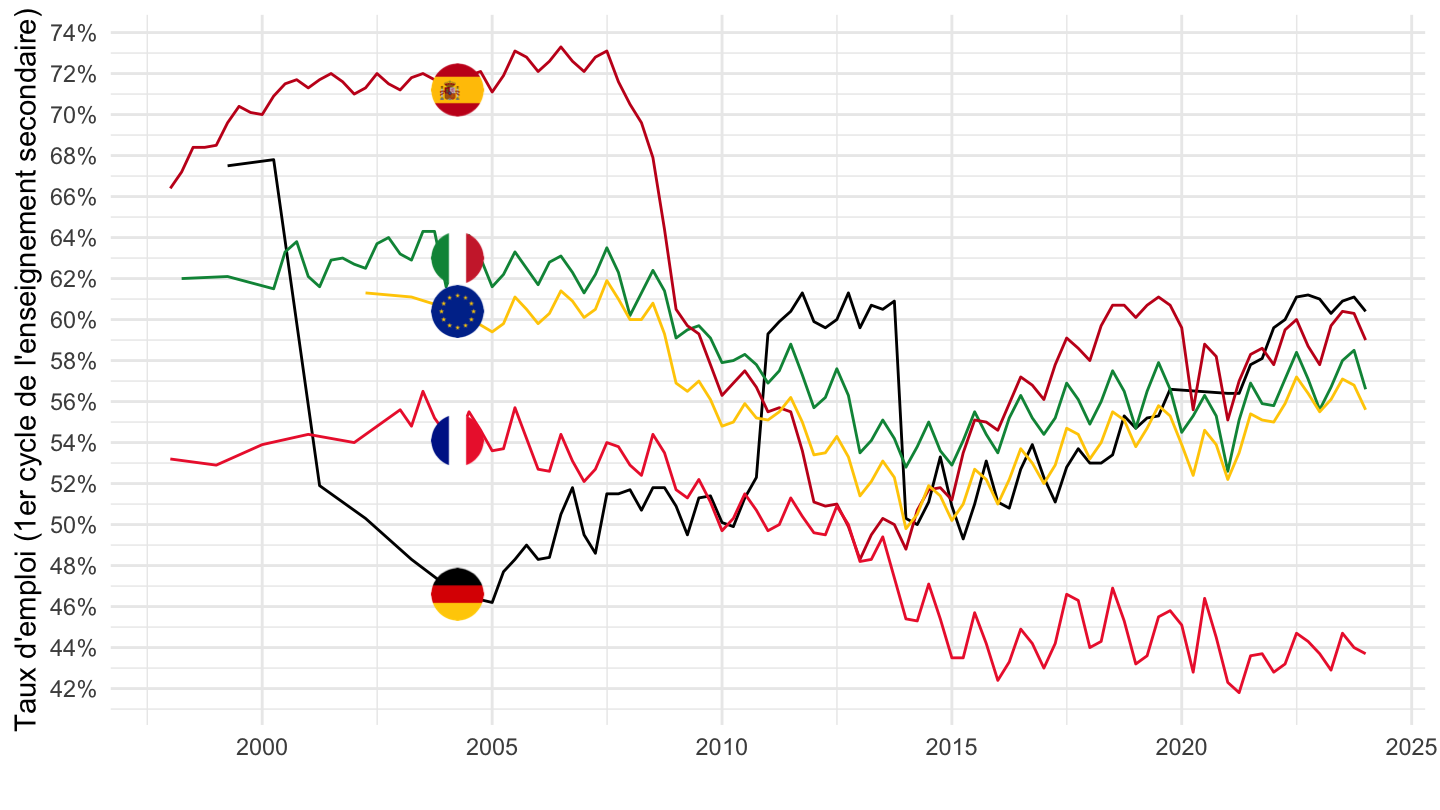
Y15-74
Code
lfsq_ergaed %>%
  filter(isced11 == "ED0-2",
         age == "Y15-74",
         geo %in% c("EA20", "DE", "ES", "FR", "IT"),
         sex == "T") %>%
  quarter_to_date() %>%
  filter(date >= as.Date("1995-01-01")) %>%

  mutate(Geo = ifelse(geo == "DE", "Germany", Geo)) %>%
  mutate(Geo = ifelse(geo == "EA20", "Europe", Geo)) %>%
  left_join(colors, by = c("Geo" = "country")) %>%
  mutate(color = ifelse(geo == "EA20", color2, color)) %>%
  mutate(color = ifelse(geo == "ES", color2, color)) %>%
  mutate(values = values / 100) %>%
  ggplot(.) + geom_line(aes(x = date, y = values, color = color)) +
  theme_minimal() + xlab("") + ylab("Taux d'emploi (1er cycle de l'enseignement secondaire)") +
  scale_color_identity() + add_5flags +
  scale_x_date(breaks = seq(1960, 2100, 5) %>% paste0("-01-01") %>% as.Date,
               labels = date_format("%Y")) +
  scale_y_continuous(breaks = 0.01*seq(-500, 200, 2),
                     labels = percent_format(accuracy = 1))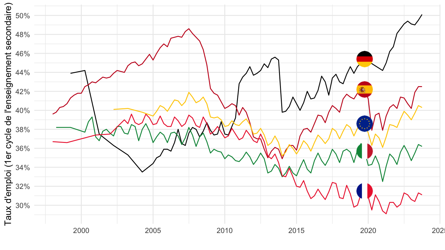
Education moyenne
Code
lfsq_ergaed %>%
  filter(isced11 == "ED3_4",
         age == "Y15-74",
         geo %in% c("EA20", "DE", "ES", "FR", "IT"),
         sex == "T") %>%
  quarter_to_date() %>%
  filter(date >= as.Date("1995-01-01")) %>%

  mutate(Geo = ifelse(geo == "DE", "Germany", Geo)) %>%
  mutate(Geo = ifelse(geo == "EA20", "Europe", Geo)) %>%
  left_join(colors, by = c("Geo" = "country")) %>%
  mutate(color = ifelse(geo == "EA20", color2, color)) %>%
  mutate(color = ifelse(geo == "ES", color2, color)) %>%
  mutate(values = values / 100) %>%
  ggplot(.) + geom_line(aes(x = date, y = values, color = color)) +
  theme_minimal() + xlab("") + ylab("Taux d'emploi") +
  scale_color_identity() + add_5flags +
  scale_x_date(breaks = seq(1960, 2100, 5) %>% paste0("-01-01") %>% as.Date,
               labels = date_format("%Y")) +
  scale_y_continuous(breaks = 0.01*seq(-500, 200, 2),
                     labels = percent_format(accuracy = 1))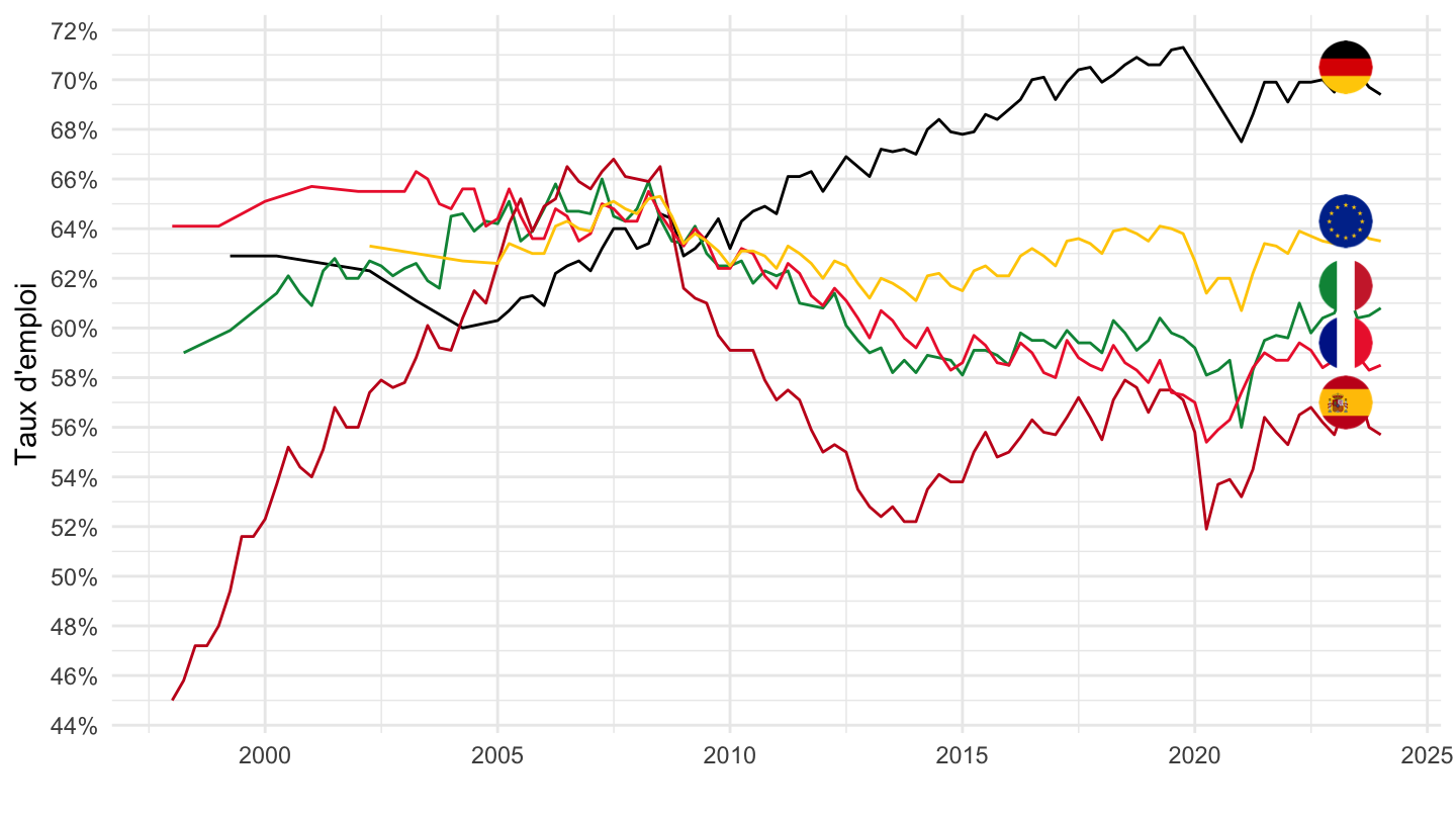
Enseignement supérieur
Code
lfsq_ergaed %>%
  filter(isced11 == "ED5-8",
         age == "Y15-74",
         geo %in% c("EA20", "DE", "ES", "FR", "IT"),
         sex == "T") %>%
  quarter_to_date() %>%
  filter(date >= as.Date("1995-01-01")) %>%

  mutate(Geo = ifelse(geo == "DE", "Germany", Geo)) %>%
  mutate(Geo = ifelse(geo == "EA20", "Europe", Geo)) %>%
  left_join(colors, by = c("Geo" = "country")) %>%
  mutate(color = ifelse(geo == "EA20", color2, color)) %>%
  mutate(color = ifelse(geo == "ES", color2, color)) %>%
  mutate(values = values / 100) %>%
  ggplot(.) + geom_line(aes(x = date, y = values, color = color)) +
  theme_minimal() + xlab("") + ylab("Taux d'emploi") +
  scale_color_identity() + add_5flags +
  scale_x_date(breaks = seq(1960, 2100, 5) %>% paste0("-01-01") %>% as.Date,
               labels = date_format("%Y")) +
  scale_y_continuous(breaks = 0.01*seq(-500, 200, 2),
                     labels = percent_format(accuracy = 1))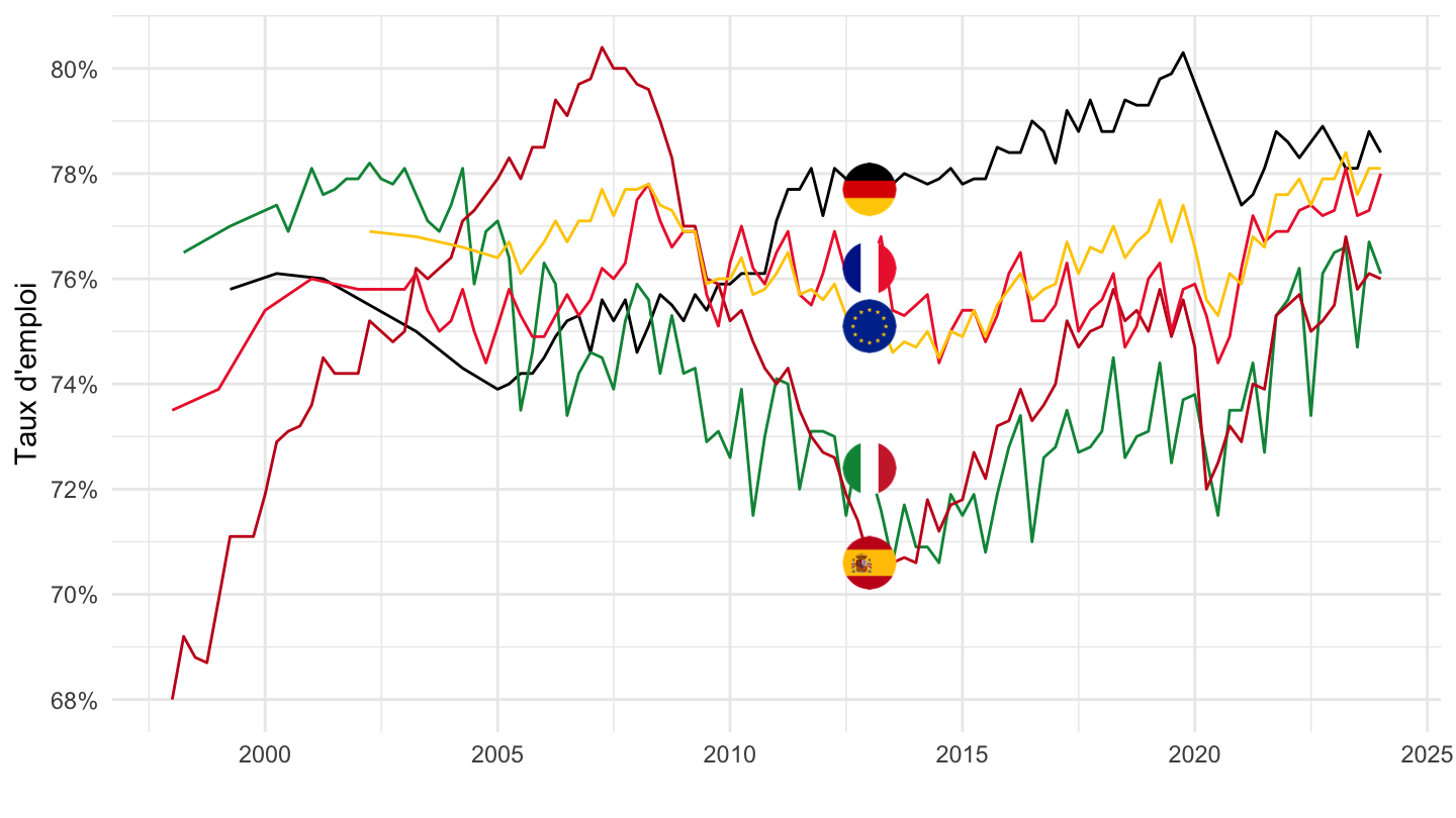
TOTAL
Code
lfsq_ergaed %>%
  filter(isced11 == "TOTAL",
         age == "Y15-74",
         geo %in% c("ES", "DE", "FR", "IT", "EA20"),
         sex == "T") %>%
  quarter_to_date() %>%
  filter(date >= as.Date("1995-01-01")) %>%

  mutate(Geo = ifelse(geo == "DE", "Germany", Geo)) %>%
  mutate(Geo = ifelse(geo == "EA20", "Europe", Geo)) %>%
  left_join(colors, by = c("Geo" = "country")) %>%
  mutate(color = ifelse(geo == "EA20", color2, color)) %>%
  mutate(color = ifelse(geo == "ES", color2, color)) %>%
  mutate(values = values / 100) %>%
  ggplot(.) + geom_line(aes(x = date, y = values, color = color)) +
  theme_minimal() + xlab("") + ylab("Taux d'emploi") +
  scale_color_identity() + add_5flags +
  scale_x_date(breaks = seq(1960, 2100, 5) %>% paste0("-01-01") %>% as.Date,
               labels = date_format("%Y")) +
  scale_y_continuous(breaks = 0.01*seq(-500, 200, 2),
                     labels = percent_format(accuracy = 1))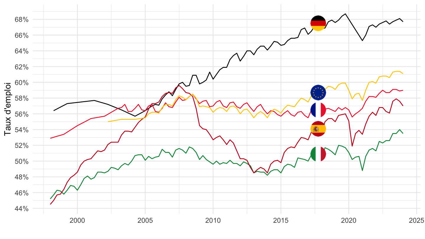
EU: Employment Rates - All
All
Code
lfsq_ergaed %>%
  filter(geo %in% c("EU15", "EU28", "EU27_2020"),
         age == "Y15-64",
         isced11 == "TOTAL",
         sex == "T",
         unit == "PC") %>%
  quarter_to_date %>%

  ggplot + geom_line() + theme_minimal()  +
  aes(x = date, y = values/100, color = Geo, linetype = Geo) +
  scale_color_manual(values = viridis(4)[1:3]) +
  scale_x_date(breaks = as.Date(paste0(seq(1960, 2100, 2), "-01-01")),
               labels = date_format("%Y")) +
  theme(legend.position = c(0.3, 0.85),
        legend.title = element_blank()) +
  xlab("") + ylab("Employment Rates") +
  scale_y_continuous(breaks = 0.01*seq(0, 200, 1),
                     labels = scales::percent_format(accuracy = 1))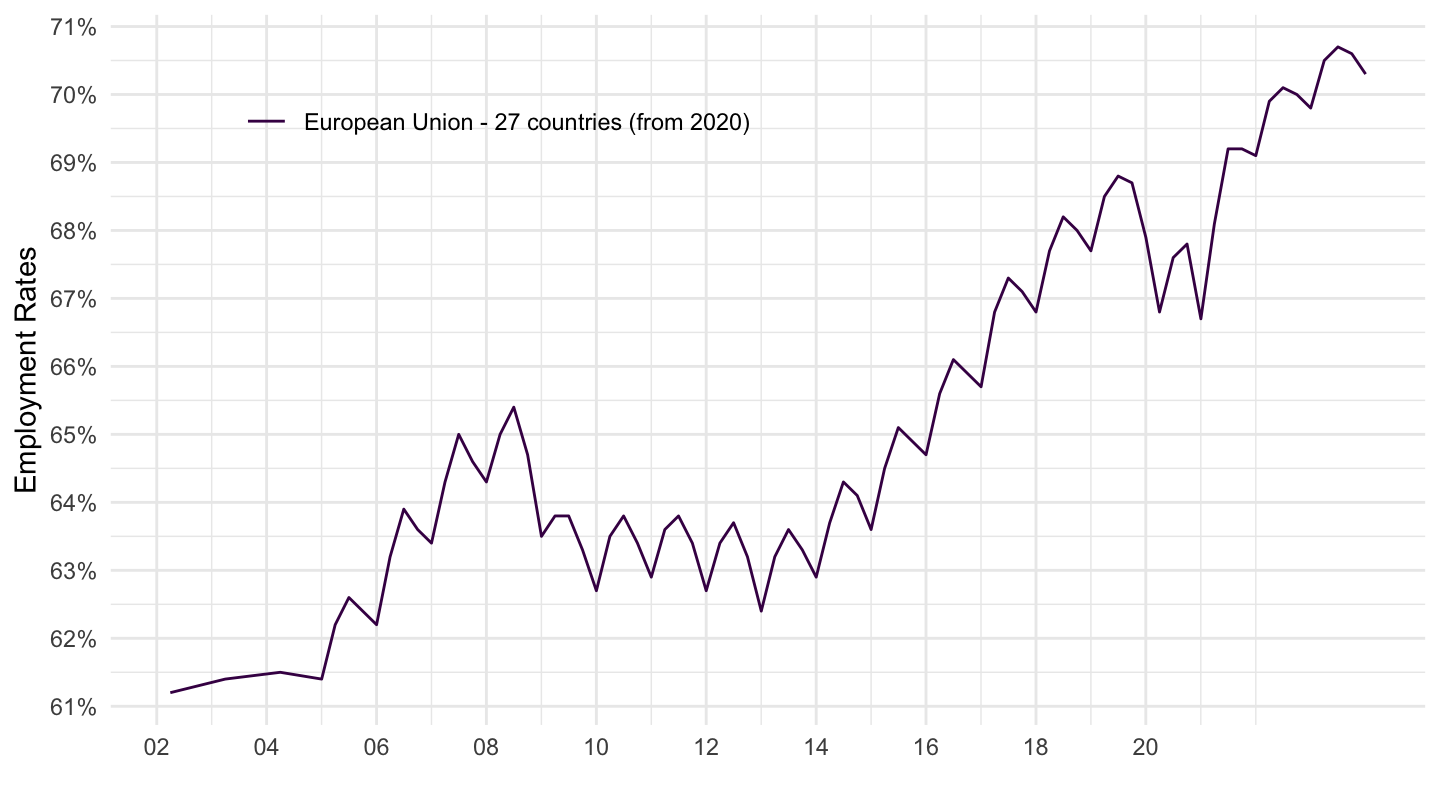
Female
Code
lfsq_ergaed %>%
  filter(geo %in% c("EU15", "EU28", "EU27_2020"),
         age == "Y15-64",
         isced11 == "TOTAL",
         sex == "F",
         unit == "PC") %>%
  quarter_to_date %>%

  ggplot + geom_line() + theme_minimal()  +
  aes(x = date, y = values/100, color = Geo, linetype = Geo) +
  scale_color_manual(values = viridis(4)[1:3]) +
  scale_x_date(breaks = as.Date(paste0(seq(1960, 2100, 2), "-01-01")),
               labels = date_format("%Y")) +
  theme(legend.position = c(0.3, 0.85),
        legend.title = element_blank()) +
  xlab("") + ylab("Employment Rates (Female)") +
  scale_y_continuous(breaks = 0.01*seq(0, 200, 1),
                     labels = scales::percent_format(accuracy = 1))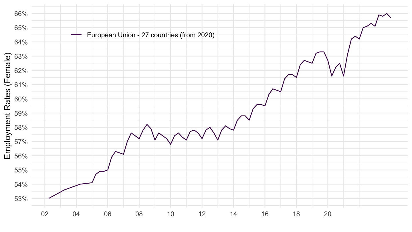
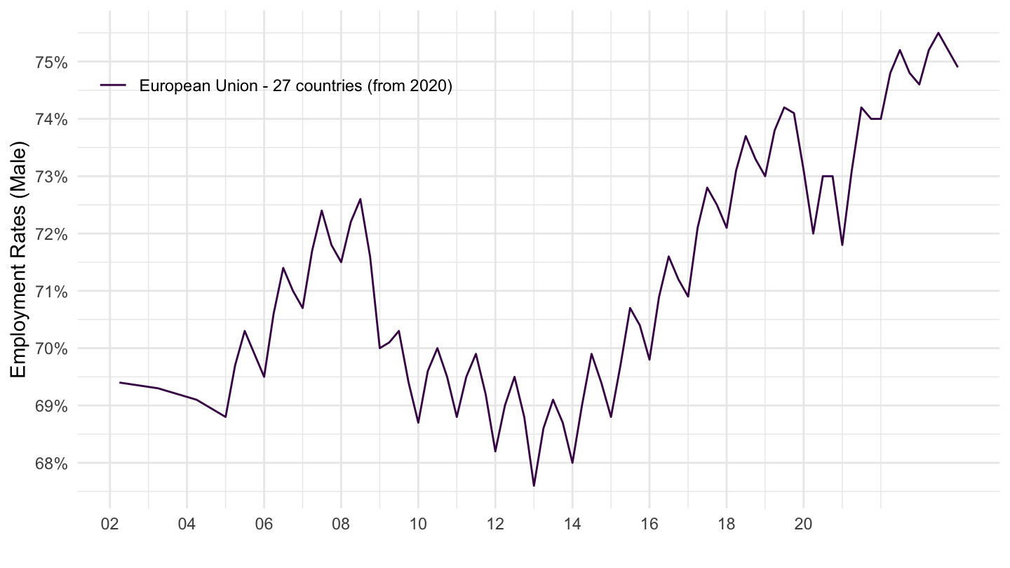
Male
Code
lfsq_ergaed %>%
  filter(geo %in% c("EU15", "EU28", "EU27_2020"),
         age == "Y15-64",
         isced11 == "TOTAL",
         sex == "M",
         unit == "PC") %>%
  quarter_to_date %>%

  ggplot + geom_line() + theme_minimal()  +
  aes(x = date, y = values/100, color = Geo, linetype = Geo) +
  scale_color_manual(values = viridis(4)[1:3]) +
  scale_x_date(breaks = as.Date(paste0(seq(1960, 2100, 2), "-01-01")),
               labels = date_format("%Y")) +
  theme(legend.position = c(0.22, 0.85),
        legend.title = element_blank()) +
  xlab("") + ylab("Employment Rates (Male)") +
  scale_y_continuous(breaks = 0.01*seq(0, 200, 1),
                     labels = scales::percent_format(accuracy = 1))