| source | dataset | Title | .html | .rData |
|---|---|---|---|---|
| eurostat | lfsa_ergaed | Employment rates by sex, age and educational attainment level (%) - lfsa_ergaed | 2026-06-03 | 2026-04-26 |
Employment rates by sex, age and educational attainment level (%) - lfsa_ergaed
Data - Eurostat
Info
LAST_COMPILE
| LAST_COMPILE |
|---|
| 2026-06-21 |
Last
Code
lfsa_ergaed %>%
  group_by(time) %>%
  summarise(Nobs = n()) %>%
  arrange(desc(time)) %>%
  head(1) %>%
print_table_conditional()| time | Nobs |
|---|---|
| 2024 | 21978 |
unit
Code
lfsa_ergaed %>%
  left_join(unit, by = "unit") %>%
  group_by(unit, Unit) %>%
  summarise(Nobs = n()) %>%
  arrange(-Nobs) %>%
print_table_conditional()| unit | Unit | Nobs |
|---|---|---|
| PC | Percentage | 486432 |
sex
Code
lfsa_ergaed %>%
  left_join(sex, by = "sex") %>%
  group_by(sex, Sex) %>%
  summarise(Nobs = n()) %>%
  arrange(-Nobs) %>%
print_table_conditional()| sex | Sex | Nobs |
|---|---|---|
| T | Total | 162617 |
| F | Females | 161926 |
| M | Males | 161889 |
age
Code
lfsa_ergaed %>%
  left_join(age, by = "age") %>%
  group_by(age, Age) %>%
  summarise(Nobs = n()) %>%
  arrange(-Nobs) %>%
  print_table_conditional()
isced11
Code
load_data("eurostat/isced11_fr.RData")
lfsa_ergaed %>%
  left_join(isced11, by = "isced11") %>%
  group_by(isced11, Isced11) %>%
  summarise(Nobs = n()) %>%
  arrange(-Nobs) %>%
print_table_conditional()| isced11 | Isced11 | Nobs |
|---|---|---|
| TOTAL | Ensemble des niveaux de la CITE 2011 | 108768 |
| ED0-2 | Inférieur à l'enseignement primaire, enseignement primaire et premier cycle de l'enseignement secondaire (niveaux 0-2) | 97617 |
| ED3_4 | Deuxième cycle de l'enseignement secondaire et enseignement post-secondaire non-supérieur (niveaux 3 et 4) | 97613 |
| ED5-8 | Enseignement supérieur (niveaux 5-8) | 96220 |
| NRP | Sans réponse | 49686 |
| ED35_45 | Deuxième cycle du secondaire et post-secondaire non-supérieur - professionnel (niveaux 35 et 45) | 18350 |
| ED34_44 | Deuxième cycle du secondaire et post-secondaire non-supérieur - général (niveaux 34 et 44) | 18106 |
| NAP | Non applicable | 72 |
geo
Code
lfsa_ergaed %>%
  left_join(geo, by = "geo") %>%
  group_by(geo, Geo) %>%
  summarise(Nobs = n()) %>%
  arrange(-Nobs) %>%
  mutate(Geo = ifelse(geo == "DE", "Germany", Geo)) %>%
  mutate(Flag = gsub(" ", "-", str_to_lower(Geo)),
         Flag = paste0('<img src="../../icon/flag/vsmall/', Flag, '.png" alt="Flag">')) %>%
  select(Flag, everything()) %>%
  {if (is_html_output()) datatable(., filter = 'top', rownames = F, escape = F) else .}
time
Code
lfsa_ergaed %>%
  group_by(time) %>%
  summarise(Nobs = n()) %>%
  arrange(desc(time)) %>%
  print_table_conditional()
France, EU, Italy, Germany, Spain, Netherlands
15-74, peu d’éducation
Code
lfsa_ergaed %>%
  filter(isced11 == "ED0-2",
         age == "Y15-74",
         geo %in% c("EA20", "DE", "ES", "FR", "IT"),
         sex == "T") %>%
  year_to_date() %>%
  filter(date >= as.Date("1995-01-01")) %>%
  left_join(geo, by = "geo") %>%
  mutate(Geo = ifelse(geo == "DE", "Germany", Geo)) %>%
  mutate(Geo = ifelse(geo == "EA20", "Europe", Geo)) %>%
  left_join(colors, by = c("Geo" = "country")) %>%
  mutate(color = ifelse(geo == "EA20", color2, color)) %>%
  mutate(color = ifelse(geo == "ES", color2, color)) %>%
  mutate(values = values / 100) %>%
  ggplot(.) + geom_line(aes(x = date, y = values, color = color)) +
  theme_minimal() + xlab("") + ylab("Taux d'emploi (1er cycle de l'enseignement secondaire)") +
  scale_color_identity() + add_5flags +
  scale_x_date(breaks = seq(1960, 2100, 5) %>% paste0("-01-01") %>% as.Date,
               labels = date_format("%Y")) +
  scale_y_continuous(breaks = 0.01*seq(-500, 200, 2),
                     labels = percent_format(accuracy = 1))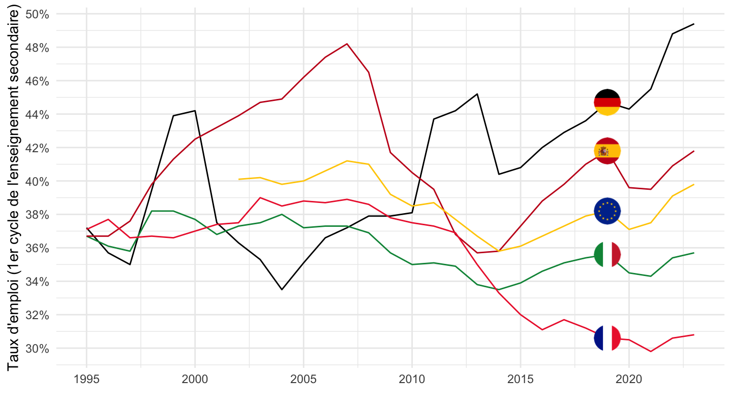
Education moyenne
Code
lfsa_ergaed %>%
  filter(isced11 == "ED3_4",
         age == "Y15-74",
         geo %in% c("EA20", "DE", "ES", "FR", "IT"),
         sex == "T") %>%
  year_to_date() %>%
  filter(date >= as.Date("1995-01-01")) %>%
  left_join(geo, by = "geo") %>%
  mutate(Geo = ifelse(geo == "DE", "Germany", Geo)) %>%
  mutate(Geo = ifelse(geo == "EA20", "Europe", Geo)) %>%
  left_join(colors, by = c("Geo" = "country")) %>%
  mutate(color = ifelse(geo == "EA20", color2, color)) %>%
  mutate(color = ifelse(geo == "ES", color2, color)) %>%
  mutate(values = values / 100) %>%
  ggplot(.) + geom_line(aes(x = date, y = values, color = color)) +
  theme_minimal() + xlab("") + ylab("Taux d'emploi") +
  scale_color_identity() + add_5flags +
  scale_x_date(breaks = seq(1960, 2100, 5) %>% paste0("-01-01") %>% as.Date,
               labels = date_format("%Y")) +
  scale_y_continuous(breaks = 0.01*seq(-500, 200, 2),
                     labels = percent_format(accuracy = 1))
Enseignement supérieur
Code
lfsa_ergaed %>%
  filter(isced11 == "ED5-8",
         age == "Y15-74",
         geo %in% c("EA20", "DE", "ES", "FR", "IT"),
         sex == "T") %>%
  year_to_date() %>%
  filter(date >= as.Date("1995-01-01")) %>%
  left_join(geo, by = "geo") %>%
  mutate(Geo = ifelse(geo == "DE", "Germany", Geo)) %>%
  mutate(Geo = ifelse(geo == "EA20", "Europe", Geo)) %>%
  left_join(colors, by = c("Geo" = "country")) %>%
  mutate(color = ifelse(geo == "EA20", color2, color)) %>%
  mutate(color = ifelse(geo == "ES", color2, color)) %>%
  mutate(values = values / 100) %>%
  ggplot(.) + geom_line(aes(x = date, y = values, color = color)) +
  theme_minimal() + xlab("") + ylab("Taux d'emploi") +
  scale_color_identity() + add_5flags +
  scale_x_date(breaks = seq(1960, 2100, 5) %>% paste0("-01-01") %>% as.Date,
               labels = date_format("%Y")) +
  scale_y_continuous(breaks = 0.01*seq(-500, 200, 2),
                     labels = percent_format(accuracy = 1))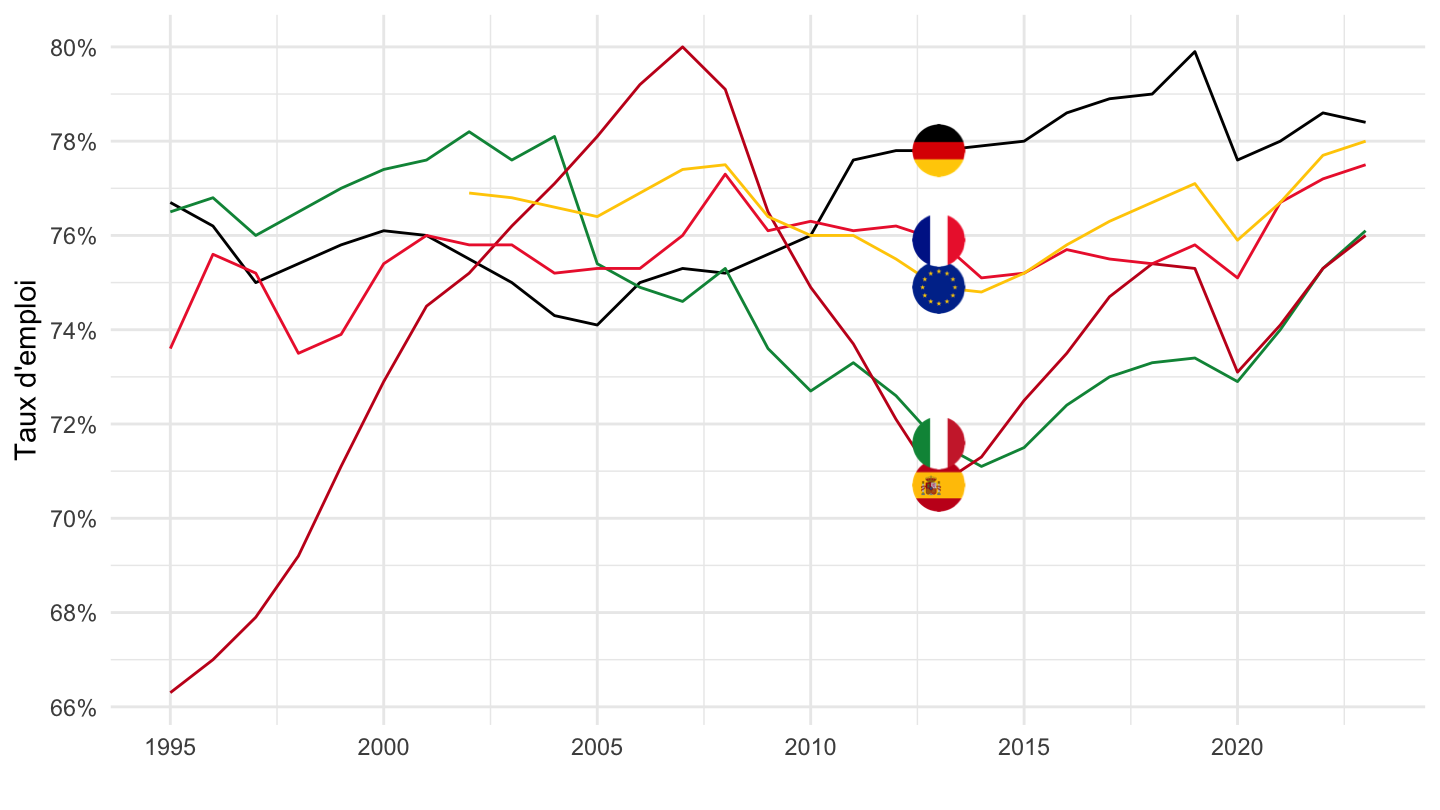
TOTAL
Code
lfsa_ergaed %>%
  filter(isced11 == "TOTAL",
         age == "Y15-74",
         geo %in% c("ES", "DE", "FR", "IT", "EA20"),
         sex == "T") %>%
  year_to_date() %>%
  filter(date >= as.Date("1995-01-01")) %>%
  left_join(geo, by = "geo") %>%
  mutate(Geo = ifelse(geo == "DE", "Germany", Geo)) %>%
  mutate(Geo = ifelse(geo == "EA20", "Europe", Geo)) %>%
  left_join(colors, by = c("Geo" = "country")) %>%
  mutate(color = ifelse(geo == "EA20", color2, color)) %>%
  mutate(color = ifelse(geo == "ES", color2, color)) %>%
  mutate(values = values / 100) %>%
  ggplot(.) + geom_line(aes(x = date, y = values, color = color)) +
  theme_minimal() + xlab("") + ylab("Taux d'emploi") +
  scale_color_identity() + add_5flags +
  scale_x_date(breaks = seq(1960, 2100, 5) %>% paste0("-01-01") %>% as.Date,
               labels = date_format("%Y")) +
  scale_y_continuous(breaks = 0.01*seq(-500, 200, 2),
                     labels = percent_format(accuracy = 1))
EU: Employment Rates - All
All
Code
lfsa_ergaed %>%
  filter(geo %in% c("EU15", "EU28", "EU27_2020"),
         age == "Y15-64",
         isced11 == "TOTAL",
         sex == "T",
         unit == "PC") %>%
  year_to_date %>%
  left_join(geo, by = "geo") %>%
  ggplot + geom_line() + theme_minimal()  +
  aes(x = date, y = values/100, color = Geo, linetype = Geo) +
  scale_color_manual(values = viridis(4)[1:3]) +
  scale_x_date(breaks = as.Date(paste0(seq(1960, 2100, 2), "-01-01")),
               labels = date_format("%Y")) +
  theme(legend.position = c(0.3, 0.85),
        legend.title = element_blank()) +
  xlab("") + ylab("Employment Rates") +
  scale_y_continuous(breaks = 0.01*seq(0, 200, 1),
                     labels = scales::percent_format(accuracy = 1))
Female
Code
lfsa_ergaed %>%
  filter(geo %in% c("EU15", "EU28", "EU27_2020"),
         age == "Y15-64",
         isced11 == "TOTAL",
         sex == "F",
         unit == "PC") %>%
  year_to_date %>%
  left_join(geo, by = "geo") %>%
  ggplot + geom_line() + theme_minimal()  +
  aes(x = date, y = values/100, color = Geo, linetype = Geo) +
  scale_color_manual(values = viridis(4)[1:3]) +
  scale_x_date(breaks = as.Date(paste0(seq(1960, 2100, 2), "-01-01")),
               labels = date_format("%Y")) +
  theme(legend.position = c(0.3, 0.85),
        legend.title = element_blank()) +
  xlab("") + ylab("Employment Rates (Female)") +
  scale_y_continuous(breaks = 0.01*seq(0, 200, 1),
                     labels = scales::percent_format(accuracy = 1))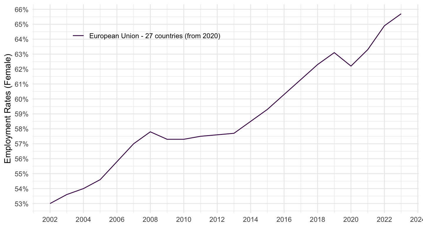
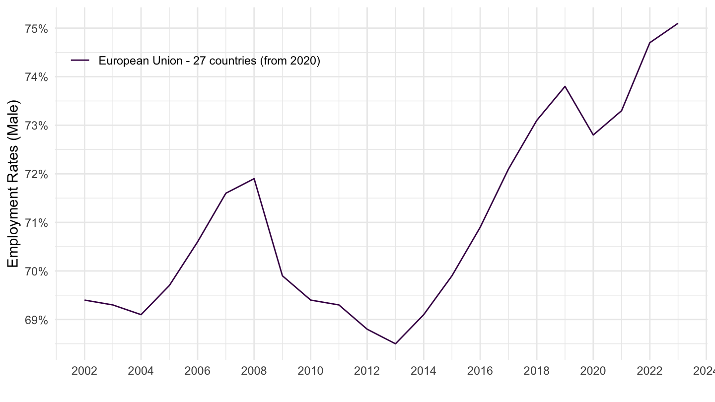
Male
Code
lfsa_ergaed %>%
  filter(geo %in% c("EU15", "EU28", "EU27_2020"),
         age == "Y15-64",
         isced11 == "TOTAL",
         sex == "M",
         unit == "PC") %>%
  year_to_date %>%
  left_join(geo, by = "geo") %>%
  ggplot + geom_line() + theme_minimal()  +
  aes(x = date, y = values/100, color = Geo, linetype = Geo) +
  scale_color_manual(values = viridis(4)[1:3]) +
  scale_x_date(breaks = as.Date(paste0(seq(1960, 2100, 2), "-01-01")),
               labels = date_format("%Y")) +
  theme(legend.position = c(0.22, 0.85),
        legend.title = element_blank()) +
  xlab("") + ylab("Employment Rates (Male)") +
  scale_y_continuous(breaks = 0.01*seq(0, 200, 1),
                     labels = scales::percent_format(accuracy = 1))