Balance of payments by country - annual data (BPM6)
Data - Eurostat
Info
Last observation: Annual: 2025 (N = 663,836)
First observation: Annual: 1982 (N = 13,223)
Last data update: 23 jul 2026, 22:36. Last compile: 24 jul 2026, 00:31
Structure
Denmark
Goods and Services
Code
bop_c6_a %>%
  filter(geo == "DK",
         stk_flow == "BAL",
         currency == "MIO_EUR",
         partner %in% c("EA19", "EXT_EA19", "WRL_REST"),
         bop_item %in% c("GS")) %>%

  left_join(B1GQ, by = c("geo", "time")) %>%
  mutate(values = values / B1GQ) %>%
  select(-B1GQ) %>%
  year_to_date %>%
  ggplot + geom_line(aes(x = date, y = values, color = Partner)) +

  theme_minimal()  + xlab("") + ylab("") +
  scale_x_date(breaks = as.Date(paste0(seq(1960, 2100, 2), "-01-01")),
               labels = date_format("%Y")) +
  theme(legend.position = c(0.25, 0.8),
        legend.title = element_blank()) +
  scale_y_continuous(breaks = 0.01*seq(-30, 30, 1),
                labels = percent_format(a = 1)) +
  geom_hline(yintercept = 0, linetype = "dashed",  color = "black")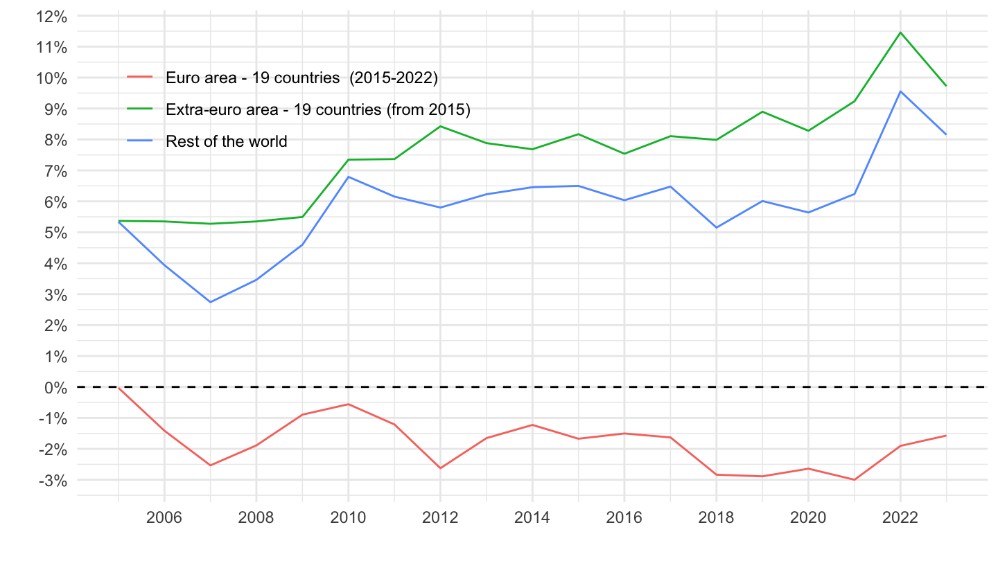
Netherlands
Goods and Services
Code
bop_c6_a %>%
  filter(geo == "NL",
         stk_flow == "BAL",
         currency == "MIO_EUR",
         partner %in% c("EA19", "EXT_EA19", "WRL_REST"),
         bop_item %in% c("GS")) %>%

  left_join(B1GQ, by = c("geo", "time")) %>%
  mutate(values = values / B1GQ) %>%
  select(-B1GQ) %>%
  year_to_date %>%
  ggplot + geom_line(aes(x = date, y = values, color = Partner)) +

  theme_minimal()  + xlab("") + ylab("") +
  scale_x_date(breaks = as.Date(paste0(seq(1960, 2100, 5), "-01-01")),
               labels = date_format("%Y")) +
  theme(legend.position = c(0.25, 0.8),
        legend.title = element_blank()) +
  scale_y_continuous(breaks = 0.01*seq(-30, 30, 1),
                labels = percent_format(a = 1)) +
  geom_hline(yintercept = 0, linetype = "dashed",  color = "black")
France
Goods and Services
Code
bop_c6_a %>%
  filter(geo == "FR",
         stk_flow == "BAL",
         currency == "MIO_EUR",
         partner %in% c("EA19", "EXT_EA19", "WRL_REST"),
         bop_item %in% c("GS")) %>%

  left_join(B1GQ, by = c("geo", "time")) %>%
  mutate(values = values / B1GQ) %>%
  select(-B1GQ) %>%
  year_to_date %>%
  ggplot + geom_line(aes(x = date, y = values, color = Partner)) +

  theme_minimal()  + xlab("") + ylab("") +
  scale_x_date(breaks = as.Date(paste0(seq(1960, 2100, 5), "-01-01")),
               labels = date_format("%Y")) +
  theme(legend.position = c(0.25, 0.8),
        legend.title = element_blank()) +
  scale_y_continuous(breaks = 0.01*seq(-30, 30, 1),
                labels = percent_format(a = 1)) +
  geom_hline(yintercept = 0, linetype = "dashed",  color = "black")
WRL_REST
Code
bop_c6_a %>%
  filter(geo == "FR",
         stk_flow == "BAL",
         currency == "MIO_EUR",
         partner %in% c("WRL_REST"),
         bop_item %in% c("CA", "GS", "G")) %>%

  left_join(B1GQ, by = c("geo", "time")) %>%
  mutate(values = values / B1GQ) %>%
  select(-B1GQ) %>%
  year_to_date %>%
  ggplot + geom_line(aes(x = date, y = values, color = Bop_item)) +

  theme_minimal()  +
  scale_x_date(breaks = as.Date(paste0(seq(1960, 2100, 5), "-01-01")),
               labels = date_format("%Y")) +
  theme(legend.position = c(0.15, 0.8),
        legend.title = element_blank()) +
  xlab("") + ylab("") +
  scale_y_continuous(breaks = 0.01*seq(-30, 30, 1),
                labels = percent_format(a = 1)) +
  geom_hline(yintercept = 0, linetype = "dashed",  color = "black")
EA19
Code
bop_c6_a %>%
  filter(geo == "FR",
         stk_flow == "BAL",
         currency == "MIO_EUR",
         partner %in% c("EA19"),
         bop_item %in% c("CA", "GS", "G")) %>%

  left_join(B1GQ, by = c("geo", "time")) %>%
  mutate(values = values / B1GQ) %>%
  select(-B1GQ) %>%
  year_to_date %>%
  ggplot + geom_line(aes(x = date, y = values, color = Bop_item)) +

  theme_minimal() + xlab("") + ylab("") +
  scale_x_date(breaks = as.Date(paste0(seq(1960, 2100, 5), "-01-01")),
               labels = date_format("%Y")) +
  theme(legend.position = c(0.15, 0.8),
        legend.title = element_blank()) +
  scale_y_continuous(breaks = 0.01*seq(-30, 30, 0.5),
                labels = percent_format(a = .1)) +
  geom_hline(yintercept = 0, linetype = "dashed",  color = "black")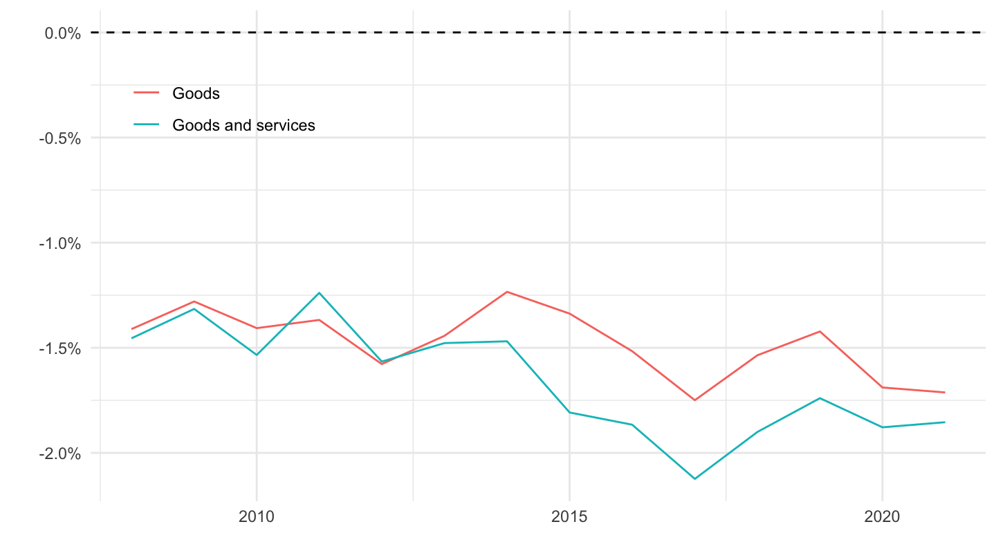
EXT_EA19
Code
bop_c6_a %>%
  filter(geo == "FR",
         stk_flow == "BAL",
         currency == "MIO_EUR",
         partner %in% c("EXT_EA19"),
         bop_item %in% c("CA", "GS", "G")) %>%

  left_join(B1GQ, by = c("geo", "time")) %>%
  mutate(values = values / B1GQ) %>%
  select(-B1GQ) %>%
  year_to_date %>%
  ggplot + geom_line(aes(x = date, y = values, color = Bop_item)) +

  theme_minimal() + xlab("") + ylab("") +
  scale_x_date(breaks = as.Date(paste0(seq(1960, 2100, 2), "-01-01")),
               labels = date_format("%Y")) +
  theme(legend.position = c(0.15, 0.8),
        legend.title = element_blank()) +
  scale_y_continuous(breaks = 0.01*seq(-30, 30, .5),
                labels = percent_format(a = .1)) +
  geom_hline(yintercept = 0, linetype = "dashed",  color = "black")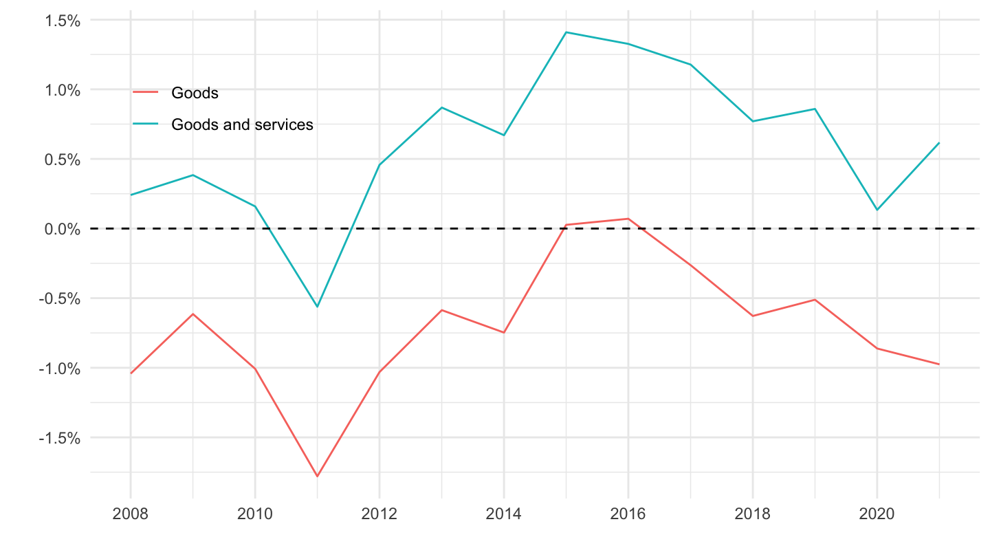
Germany
Goods and Services
Code
bop_c6_a %>%
  filter(geo == "DE",
         stk_flow == "BAL",
         currency == "MIO_EUR",
         partner %in% c("EA19", "EXT_EA19", "WRL_REST"),
         bop_item %in% c("GS")) %>%

  left_join(B1GQ, by = c("geo", "time")) %>%
  mutate(values = values / B1GQ) %>%
  select(-B1GQ) %>%
  year_to_date %>%
  ggplot + geom_line(aes(x = date, y = values, color = Partner)) +

  theme_minimal()  + xlab("") + ylab("") +
  scale_x_date(breaks = as.Date(paste0(seq(1960, 2100, 5), "-01-01")),
               labels = date_format("%Y")) +
  theme(legend.position = c(0.25, 0.8),
        legend.title = element_blank()) +
  scale_y_continuous(breaks = 0.01*seq(-30, 30, 1),
                labels = percent_format(a = 1)) +
  geom_hline(yintercept = 0, linetype = "dashed",  color = "black")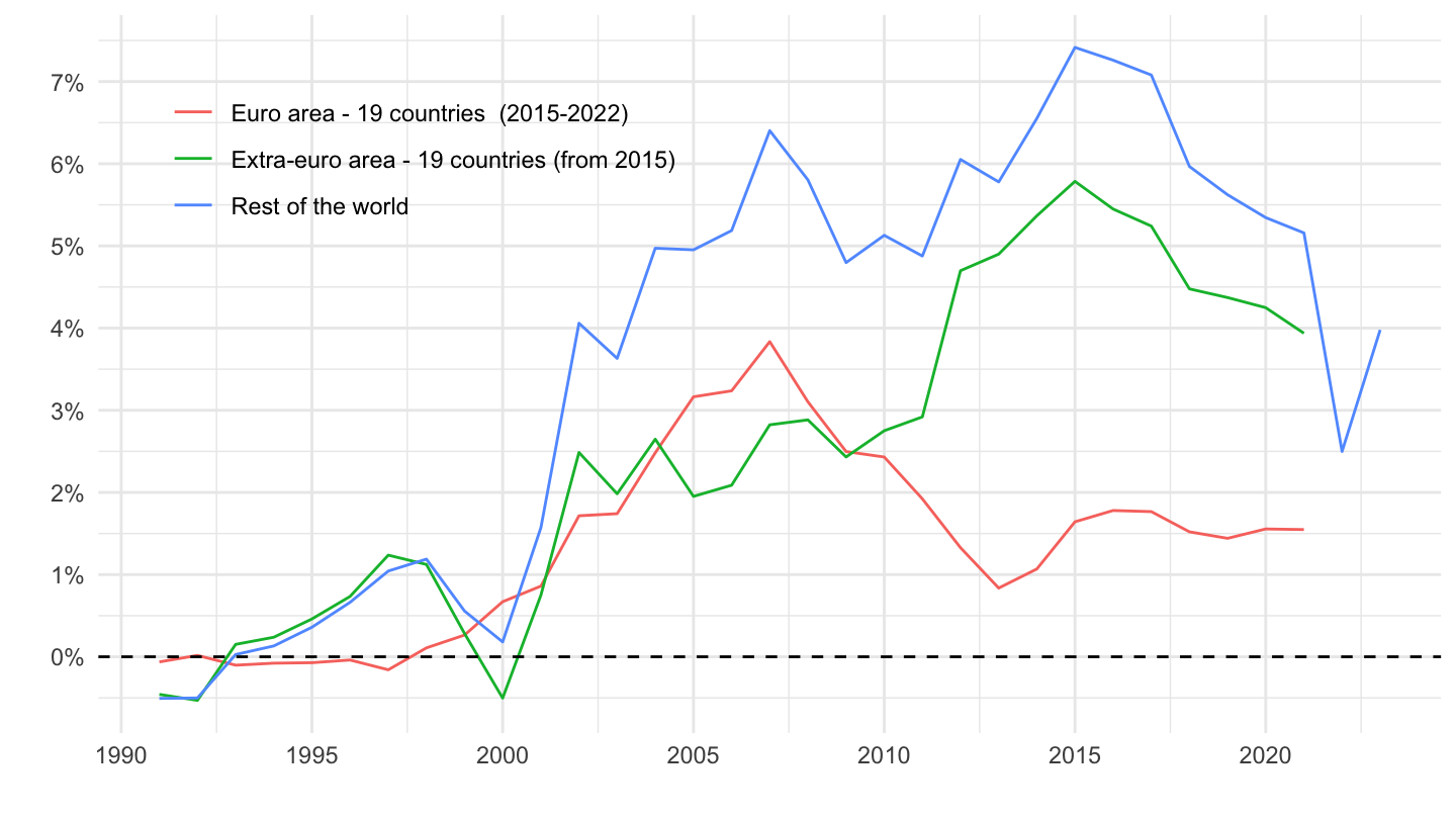
WRL_REST
Code
bop_c6_a %>%
  filter(geo == "DE",
         stk_flow == "BAL",
         currency == "MIO_EUR",
         partner %in% c("WRL_REST"),
         bop_item %in% c("CA", "GS", "G")) %>%

  left_join(B1GQ, by = c("geo", "time")) %>%
  mutate(values = values / B1GQ) %>%
  select(-B1GQ) %>%
  year_to_date %>%
  ggplot + geom_line(aes(x = date, y = values, color = Bop_item)) +

  theme_minimal()  +
  scale_x_date(breaks = as.Date(paste0(seq(1960, 2100, 5), "-01-01")),
               labels = date_format("%Y")) +
  theme(legend.position = c(0.15, 0.8),
        legend.title = element_blank()) +
  xlab("") + ylab("") +
  scale_y_continuous(breaks = 0.01*seq(-30, 30, 2),
                labels = percent_format(a = 1)) +
  geom_hline(yintercept = 0, linetype = "dashed",  color = "black")
EA19
Code
bop_c6_a %>%
  filter(geo == "DE",
         stk_flow == "BAL",
         currency == "MIO_EUR",
         partner %in% c("EA19"),
         bop_item %in% c("CA", "GS", "G")) %>%

  left_join(B1GQ, by = c("geo", "time")) %>%
  mutate(values = values / B1GQ) %>%
  select(-B1GQ) %>%
  year_to_date %>%
  ggplot + geom_line(aes(x = date, y = values, color = Bop_item)) +

  theme_minimal() + xlab("") + ylab("") +
  scale_x_date(breaks = as.Date(paste0(seq(1960, 2100, 5), "-01-01")),
               labels = date_format("%Y")) +
  theme(legend.position = c(0.15, 0.8),
        legend.title = element_blank()) +
  scale_y_continuous(breaks = 0.01*seq(-30, 30, 1),
                labels = percent_format(a = 1)) +
  geom_hline(yintercept = 0, linetype = "dashed",  color = "black")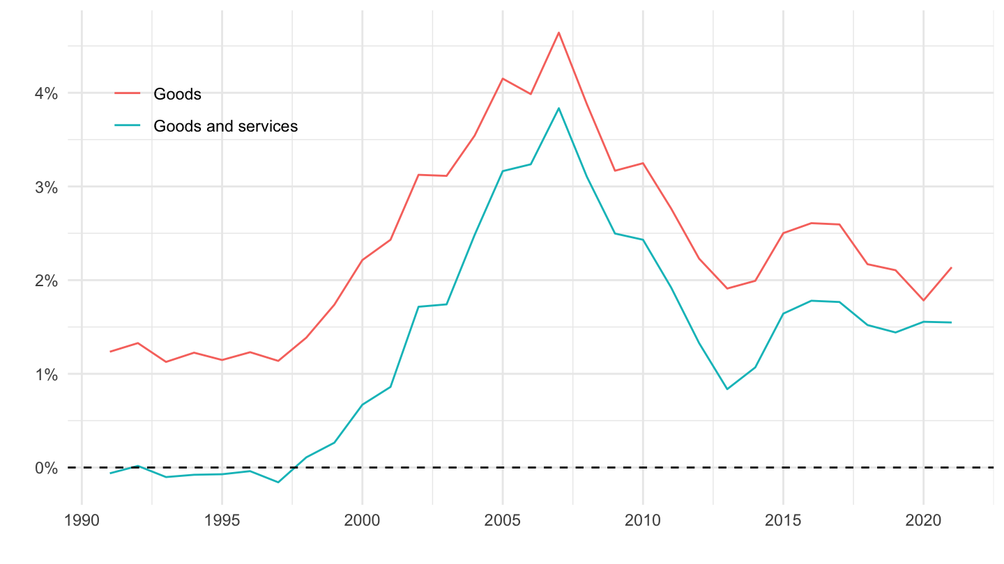
EXT_EA19
Code
bop_c6_a %>%
  filter(geo == "DE",
         stk_flow == "BAL",
         currency == "MIO_EUR",
         partner %in% c("EXT_EA19"),
         bop_item %in% c("CA", "GS", "G")) %>%

  left_join(B1GQ, by = c("geo", "time")) %>%
  mutate(values = values / B1GQ) %>%
  select(-B1GQ) %>%
  year_to_date %>%
  ggplot + geom_line(aes(x = date, y = values, color = Bop_item)) +

  theme_minimal() + xlab("") + ylab("") +
  scale_x_date(breaks = as.Date(paste0(seq(1960, 2100, 5), "-01-01")),
               labels = date_format("%Y")) +
  theme(legend.position = c(0.15, 0.8),
        legend.title = element_blank()) +
  scale_y_continuous(breaks = 0.01*seq(-30, 30, 1),
                labels = percent_format(a = 1)) +
  geom_hline(yintercept = 0, linetype = "dashed",  color = "black")