Balance of Payments - BPM6
Data - Banque de France
Info
Last observation: Mensuel: 31 mai 2026 (N = 38,801) · Trimestriel: 31 mar 2026 (N = 57,470) · Annuel: 31 déc 2025 (N = 25,896)
First observation: Mensuel: 31 jan 2013 (N = 38,801) · Trimestriel: 31 mar 2013 (N = 57,470) · Annuel: 31 déc 2013 (N = 25,896)
Last data update: 10 aoû 2026, 18:48. Last compile: 13 aoû 2026, 00:08
Structure
| source | dataset | Title | .html | .rData |
|---|---|---|---|---|
| bdf | BPM6 | Balance des paiements - 6ème manuel | 2026-08-11 | 2026-08-10 |
| eurostat | bop_iip6_q | NA | NA | NA |
Balance of Payments of France
November 2024
October 2024
Current account balance
Code
ig_b("bdf", "FR_Stat_Info_Balance_des_paiements_de_la_France_202410", "balance-courante")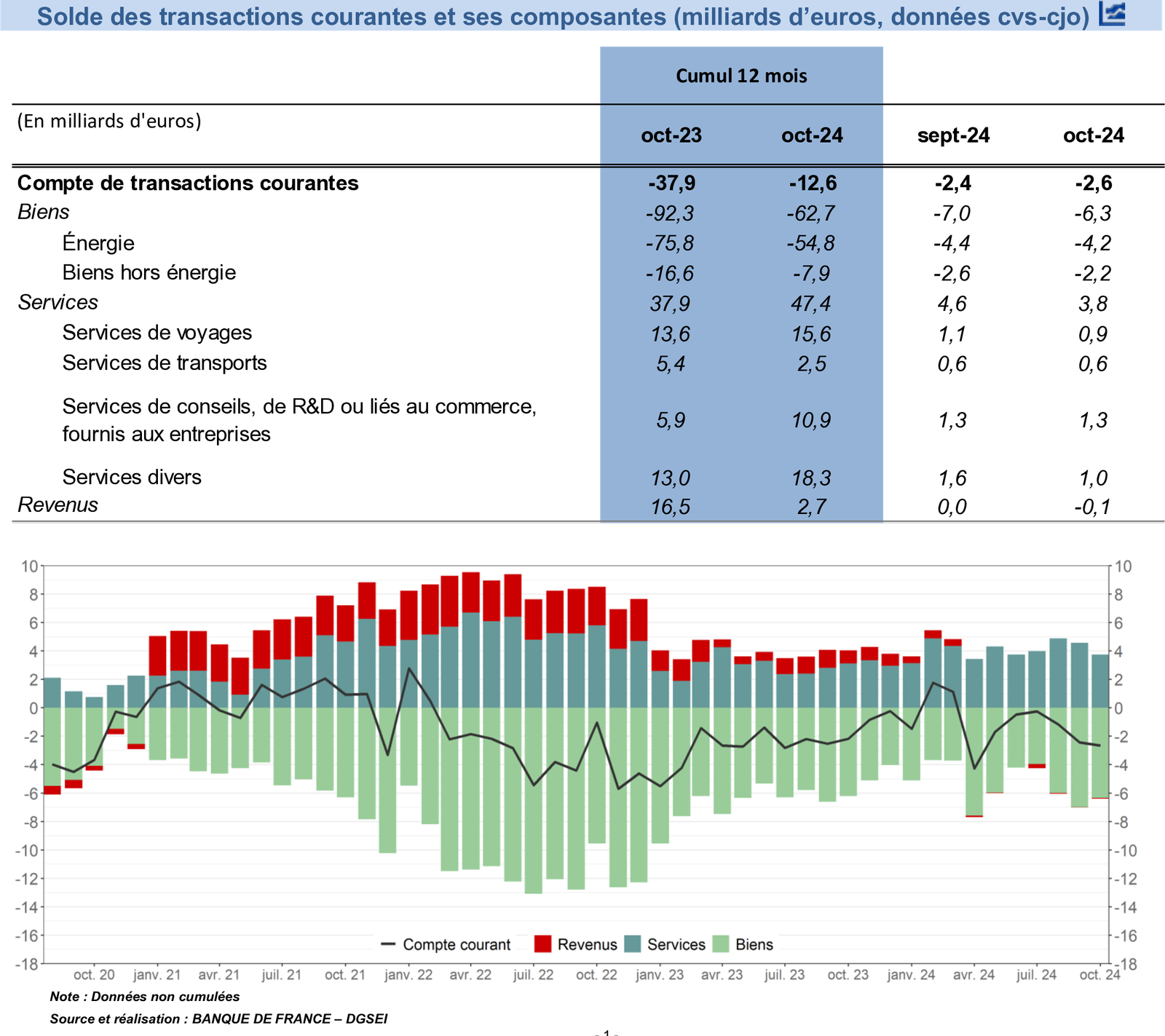
Financial account balance
Code
ig_b("bdf", "FR_Stat_Info_Balance_des_paiements_de_la_France_202410", "solde-des-operations-financieres")
January 2024
Current Account
Table
Code
ig_b("bdf", "BDP_FRA_2284_fr__BDP_Stat_Info_janvier_2024_FR", "table1")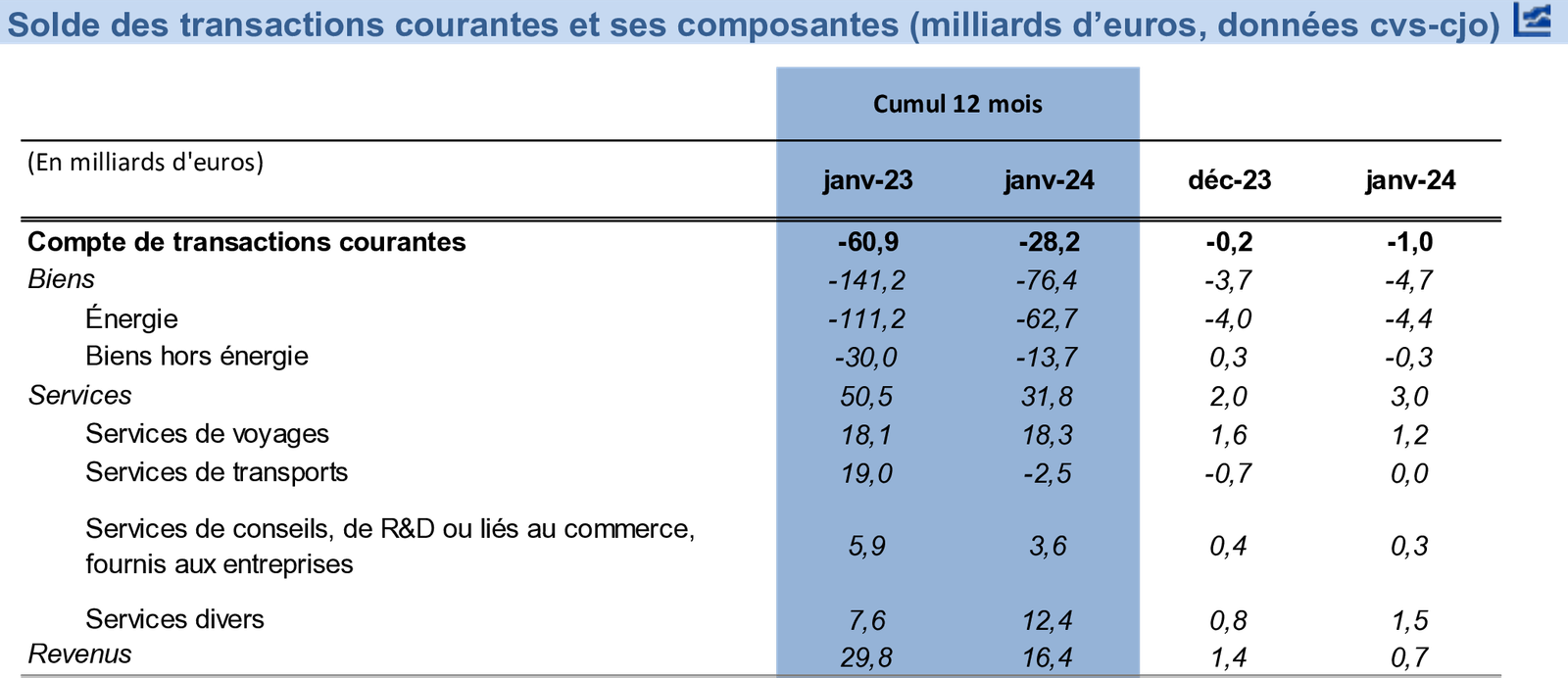
Figure
Code
ig_b("bdf", "BDP_FRA_2284_fr__BDP_Stat_Info_janvier_2024_FR", "figure1")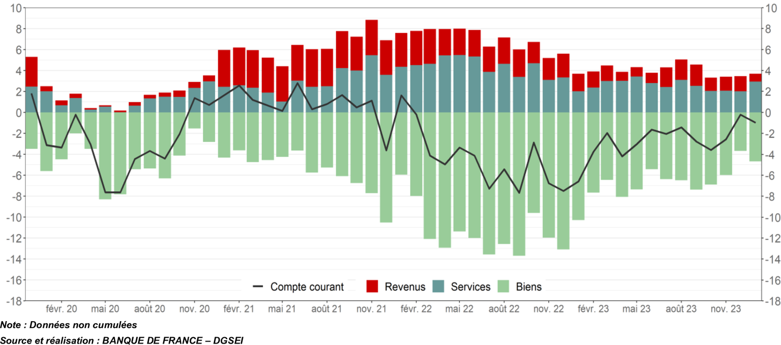
Financial Account
Table
Code
ig_b("bdf", "BDP_FRA_2284_fr__BDP_Stat_Info_janvier_2024_FR", "table2")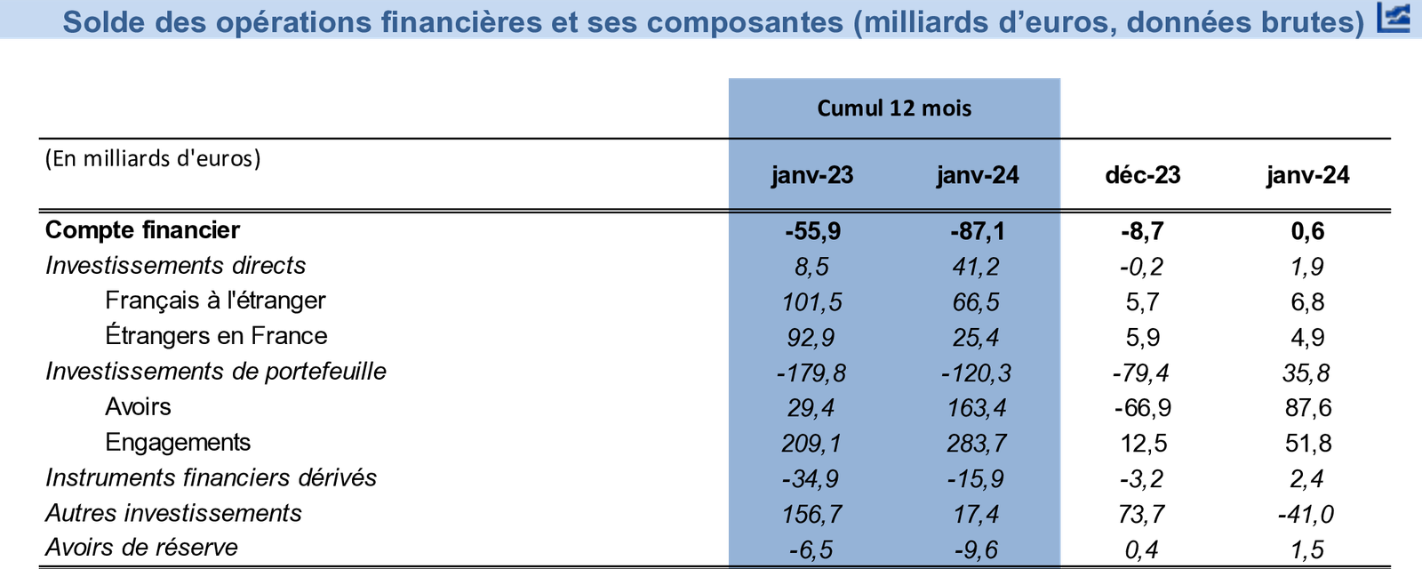
Figure
Code
ig_b("bdf", "BDP_FRA_2284_fr__BDP_Stat_Info_janvier_2024_FR", "figure2")
November 2021
Code
ig_b("bdf", "bdp_fra_2241_fr_bdp_stat_info_septembre_2021_fr", "comptes")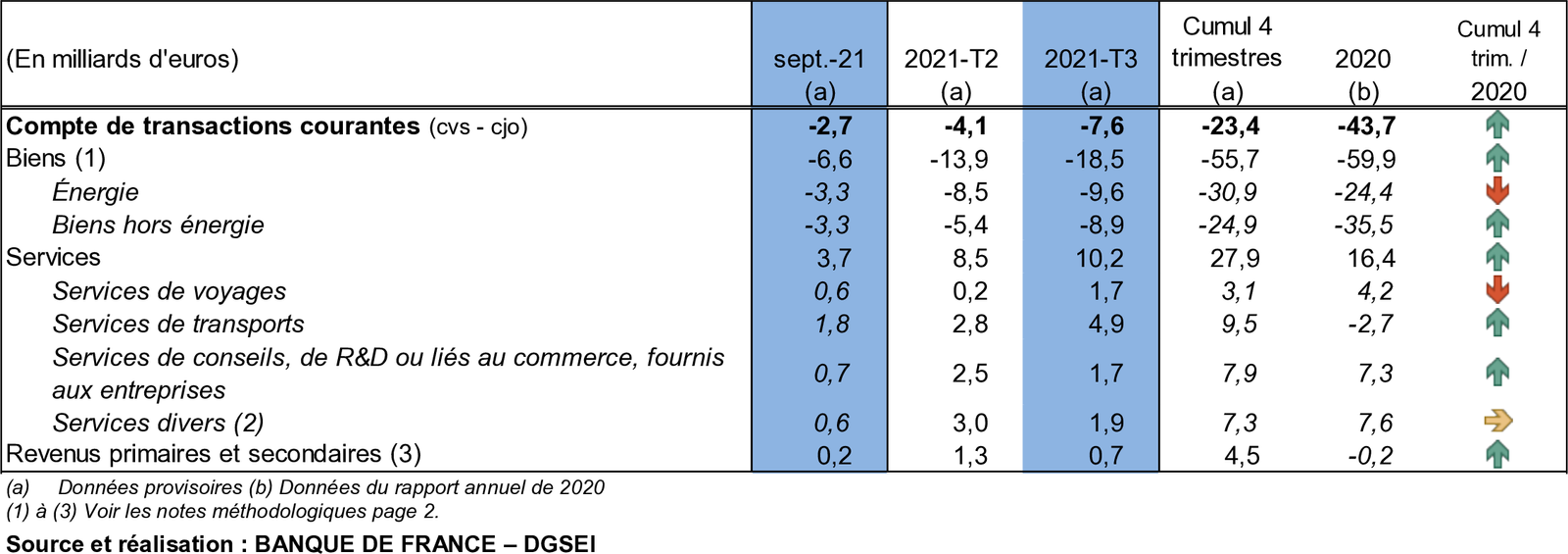
May 2020
Code
ig_b("bdf", "BPM6-2021-07")
November 2020
Code
ig_b("bdf", "BPM6-2020-11-compte")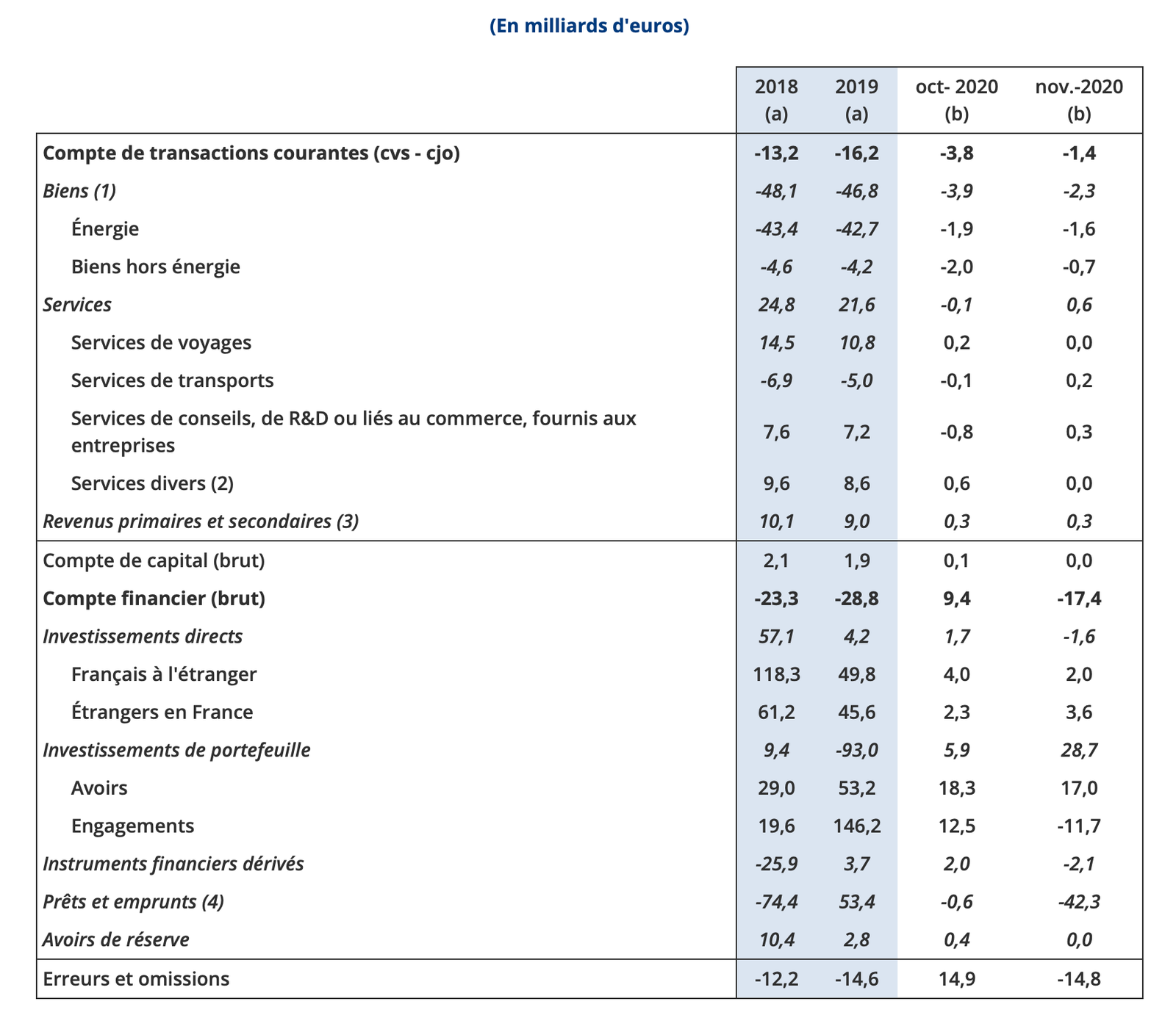
Financial account vs current account, Difference
Financial account and current account
Code
BPM6 |>

  filter(variable == "BPM6.M.N.FR.W1.S1.S1.T.N.FA._T.F._Z.EUR._T.V.N.ALL" |
           variable == "BPM6.M.S.FR.W1.S1.S1.T.B.CA._Z._Z._Z.EUR._T._X.N.ALL") |>


  group_by(Accounting_entry) |>
  arrange(date) |>
  mutate(value = zoo::rollsum(x = value, 12, align = "right", fill = NA)) |>
  na.omit() |>
  mutate(Int_acc_item = ifelse(Int_acc_item == "Transactions courantes", "Current account", Int_acc_item)) |>
   ggplot() + geom_line(aes(x = date, y = value/1000, color = Int_acc_item)) +
  scale_x_date(breaks = "1 year",
               labels = date_format("%Y")) +
  scale_y_continuous(labels = dollar_format(pre = "", su = " bn €"),
                     breaks = seq(-300000, 300000, 10000)/1000) +
  theme_minimal() + xlab("") + ylab("12-month cumulative") +
  theme(legend.position = c(0.2, 0.3),
        legend.title = element_blank(),
        legend.direction = "vertical") +
  geom_label(data = . %>% filter(date == max(date)),
             aes(x = date, y = value/1000, label = paste0(round(value/1000, 1)), color = Int_acc_item)) +
  geom_hline(yintercept = 0, linetype = "dashed")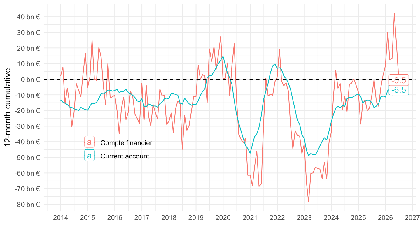
Difference
Code
BPM6 |>

  filter(variable == "BPM6.M.N.FR.W1.S1.S1.T.N.FA._T.F._Z.EUR._T.V.N.ALL" |
           variable == "BPM6.M.S.FR.W1.S1.S1.T.B.CA._Z._Z._Z.EUR._T._X.N.ALL") |>


  group_by(Accounting_entry) |>
  arrange(date) |>
  mutate(value = zoo::rollsum(x = value, 12, align = "right", fill = NA)) |>
  ungroup() |>
  select(date, value, Int_acc_item) |>
  na.omit() |>
  spread(Int_acc_item, value) |>
  mutate(`Difference` = `Compte financier` - `Transactions courantes`) |>
  gather(Int_acc_item, value, -date) |>
   ggplot() + geom_line(aes(x = date, y = value/1000, color = Int_acc_item)) +
  scale_x_date(breaks = "1 year",
               labels = date_format("%Y")) +
  scale_y_continuous(labels = dollar_format(pre = ""),
                     breaks = seq(-300000, 300000, 10000)/1000) +
  theme_minimal() + xlab("") + ylab("") +
  theme(legend.position = c(0.2, 0.3),
        legend.title = element_blank(),
        legend.direction = "vertical") +
  geom_label(data = . %>% filter(date == max(date)),
             aes(x = date, y = value/1000, label = round(value/1000, 1), color = Int_acc_item))
Foreign Direct Investment
Flows
All
Monthly
Code
BPM6 |>

  filter(variable == "BPM6.M.N.FR.W1.S1.S1.T.A.FA.D.F._Z.EUR._T.V.N.ALL" |
           variable == "BPM6.M.N.FR.W1.S1.S1.T.L.FA.D.F._Z.EUR._T.V.N.ALL" |
           variable == "BPM6.M.N.FR.W1.S1.S1.T.N.FA.D.F._Z.EUR._T.V.N.ALL") |>


  group_by(Accounting_entry) |>
  arrange(date) |>
  mutate(value = zoo::rollsum(x = value, 36, align = "right", fill = NA)/3) |>
  na.omit() |>
   ggplot() + geom_line(aes(x = date, y = value, color = Accounting_entry)) +
  scale_x_date(breaks = "1 year",
               labels = date_format("%Y")) +
  scale_y_continuous(labels = dollar_format(pre = ""),
                     breaks = seq(-10000, 300000, 5000)) +
  theme_minimal() + xlab("") + ylab("") +
  theme(legend.position = c(0.2, 0.8),
        legend.title = element_blank(),
        legend.direction = "vertical")
Quarterly
Code
BPM6 |>

  filter(variable == "BPM6.Q.N.FR.W1.S1.S1.T.A.FA.D.F._Z.EUR._T.V.N.ALL" |
           variable == "BPM6.Q.N.FR.W1.S1.S1.T.L.FA.D.F._Z.EUR._T.V.N.ALL" |
           variable == "BPM6.Q.N.FR.W1.S1.S1.T.N.FA.D.F._Z.EUR._T.V.N.ALL") |>


  group_by(Accounting_entry) |>
  arrange(date) |>
  mutate(value = zoo::rollsum(x = value, 12, align = "right", fill = NA)/3) |>
  na.omit() |>
   ggplot() + geom_line(aes(x = date, y = value, color = Accounting_entry)) +
  scale_x_date(breaks = "1 year",
               labels = date_format("%Y")) +
  scale_y_continuous(labels = dollar_format(pre = ""),
                     breaks = seq(-10000, 300000, 5000)) +
  theme_minimal() + xlab("") + ylab("") +
  theme(legend.position = c(0.2, 0.8),
        legend.title = element_blank(),
        legend.direction = "vertical")
Annual
Code
BPM6 |>

  filter(variable == "BPM6.A.N.FR.W1.S1.S1.T.A.FA.D.F._Z.EUR._T.V.N.ALL" |
           variable == "BPM6.A.N.FR.W1.S1.S1.T.L.FA.D.F._Z.EUR._T.V.N.ALL" |
           variable == "BPM6.A.N.FR.W1.S1.S1.T.N.FA.D.F._Z.EUR._T.V.N.ALL") |>


  group_by(Accounting_entry) |>
  arrange(date) |>
  mutate(value = zoo::rollsum(x = value, 4, align = "right", fill = NA)/4) |>
  na.omit() |>
   ggplot() + geom_line(aes(x = date, y = value, color = Accounting_entry)) +
  scale_x_date(breaks = "1 year",
               labels = date_format("%Y")) +
  scale_y_continuous(labels = dollar_format(pre = ""),
                     breaks = seq(-10000, 300000, 5000)) +
  theme_minimal() + xlab("") + ylab("") +
  theme(legend.position = c(0.2, 0.8),
        legend.title = element_blank(),
        legend.direction = "vertical")
2017
Code
BPM6 |>

  filter(variable == "BPM6.M.N.FR.W1.S1.S1.T.A.FA.D.F._Z.EUR._T.V.N.ALL" |
           variable == "BPM6.M.N.FR.W1.S1.S1.T.L.FA.D.F._Z.EUR._T.V.N.ALL" |
           variable == "BPM6.M.N.FR.W1.S1.S1.T.N.FA.D.F._Z.EUR._T.V.N.ALL",
            date >= as.Date("2017-01-01")) |>


  arrange(desc(date)) |>
   ggplot() + geom_line(aes(x = date, y = value, color = Accounting_entry)) +
  scale_x_date(breaks = "1 year",
               labels = date_format("%Y")) +
  theme_minimal() + xlab("") + ylab("") +
  theme(legend.position = c(0.2, 0.2),
        legend.title = element_blank(),
        legend.direction = "vertical")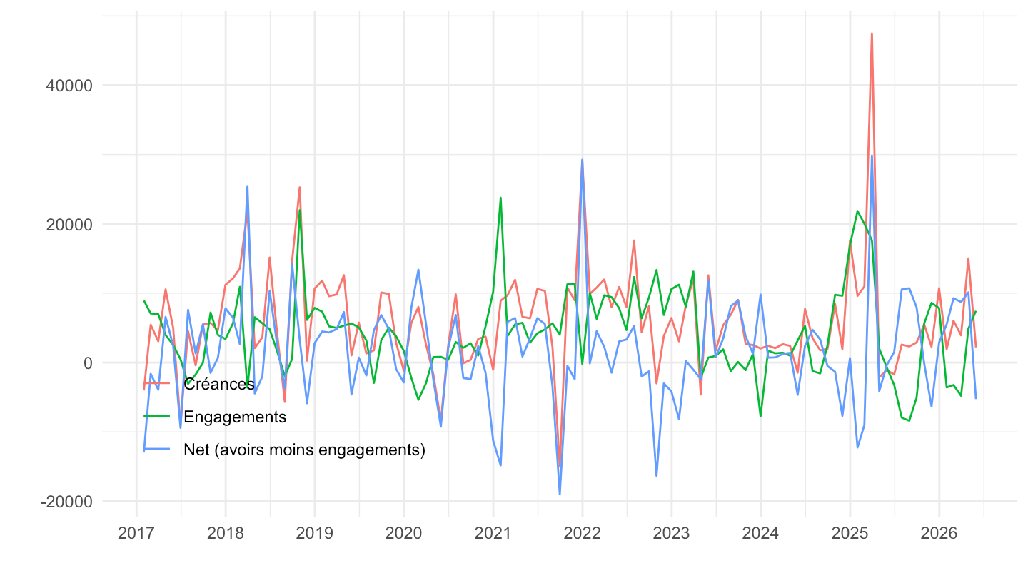
Current Account
Goods, Services, Goods & Services
Annual
Code
BPM6 |>

  filter(variable == "BPM6.A.N.FR.W1.S1.S1.T.B.G._Z._Z._Z.EUR._T._X.N.ALL" |
         variable == "BPM6.A.N.FR.W1.S1.S1.T.B.GS._Z._Z._Z.EUR._T._X.N.ALL" |
         variable == "BPM6.A.N.FR.W1.S1.S1.T.B.S._Z._Z._Z.EUR._T._X.N.ALL" |
         variable == "BPM6.A.N.FR.W1.S1.S1.T.B.CA._Z._Z._Z.EUR._T._X.N.ALL") |>

  left_join(gdp, by = "date") |>
  ggplot() + geom_line(aes(x = date, y = value /gdp / 1000, color = Int_acc_item)) +

  theme_minimal() +
  scale_x_date(breaks = "2 years",
               labels = date_format("%Y")) +
  theme(legend.position = c(0.2, 0.2),
        legend.title = element_blank(),
        legend.direction = "vertical") +
  xlab("") + ylab("Goods, Services, Goods and Services (Net)") +
  scale_y_continuous(breaks = 0.01*seq(-200, 200, 1),
                labels = percent_format(accuracy = 1))
Quarterly
Code
BPM6 |>

  filter(variable %in%c("BPM6.Q.N.FR.W1.S1.S1.T.B.GS._Z._Z._Z.EUR._T._X.N.ALL",
                        "BPM6.Q.N.FR.W1.S1.S1.T.B.G._Z._Z._Z.EUR._T._X.N.ALL",
                        "BPM6.Q.N.FR.W1.S1.S1.T.B.S._Z._Z._Z.EUR._T._X.N.ALL",
                        "BPM6.Q.N.FR.W1.S1.S1.T.B.CA._Z._Z._Z.EUR._T._X.N.ALL")) |>

  left_join(gdp_quarterly, by = "date") |>
  ggplot() + geom_line(aes(x = date, y = value/gdp, color = Int_acc_item)) +

  theme_minimal() +
  scale_x_date(breaks = "2 years",
               labels = date_format("%Y")) +
  theme(legend.position = c(0.2,0.2),
        legend.title = element_blank(),
        legend.direction = "vertical") +
  xlab("") + ylab("Balance") +
  scale_y_continuous(breaks = 0.01*seq(-200, 200, 1),
                labels = percent_format(accuracy = 1))
Monthly
Per month
Code
BPM6 |>

  filter(variable == "BPM6.M.S.FR.W1.S1.S1.T.B.GS._Z._Z._Z.EUR._T._X.N.ALL" |
         variable == "BPM6.M.S.FR.W1.S1.S1.T.B.G._Z._Z._Z.EUR._T._X.N.ALL" |
         variable == "BPM6.M.S.FR.W1.S1.S1.T.B.S._Z._Z._Z.EUR._T._X.N.ALL" |
           variable == "BPM6.M.S.FR.W1.S1.S1.T.B.CA._Z._Z._Z.EUR._T._X.N.ALL") |>

  ggplot() + geom_line(aes(x = date, y = value / 1000, color = Int_acc_item)) +

  theme_minimal() +
  scale_x_date(breaks = "1 year",
               labels = date_format("%Y")) +
  theme(legend.position = c(0.2,0.9),
        legend.title = element_blank(),
        legend.direction = "vertical") +
  xlab("") + ylab("Per month") +
  scale_y_continuous(breaks = seq(-200, 200, 2),
                labels = dollar_format(suffix = " bn €",  accuracy = 1, prefix = ""))
12-month cumulative
Code
BPM6 |>

  filter(variable == "BPM6.M.S.FR.W1.S1.S1.T.B.GS._Z._Z._Z.EUR._T._X.N.ALL" |
         variable == "BPM6.M.S.FR.W1.S1.S1.T.B.G._Z._Z._Z.EUR._T._X.N.ALL" |
         variable == "BPM6.M.S.FR.W1.S1.S1.T.B.S._Z._Z._Z.EUR._T._X.N.ALL" |
           variable == "BPM6.M.S.FR.W1.S1.S1.T.B.CA._Z._Z._Z.EUR._T._X.N.ALL") |>

  group_by(Int_acc_item) |>
  arrange(desc(date)) |>
  mutate(value = zoo::rollsum(value, 12, align = "left", fill = NA)) |>
  na.omit() |>
  ggplot() + geom_line(aes(x = date, y = value / 1000, color = Int_acc_item)) +

  theme_minimal() +
  scale_x_date(breaks = "1 year",
               labels = date_format("%Y")) +
  theme(legend.position = c(0.3, 0.2),
        legend.title = element_blank(),
        legend.direction = "vertical") +
  xlab("") + ylab("12-month cumulative") +
  scale_y_continuous(breaks = seq(-200, 200, 10),
                labels = dollar_format(suffix = " bn €",  accuracy = 1, prefix = "")) +
  geom_hline(yintercept = 0, linetype = "dashed") +
  geom_label_repel(data = . %>% filter(date == max(date)),
             aes(x = date, y = value/1000, color = Int_acc_item, label = round(value/1000, digits = 1)))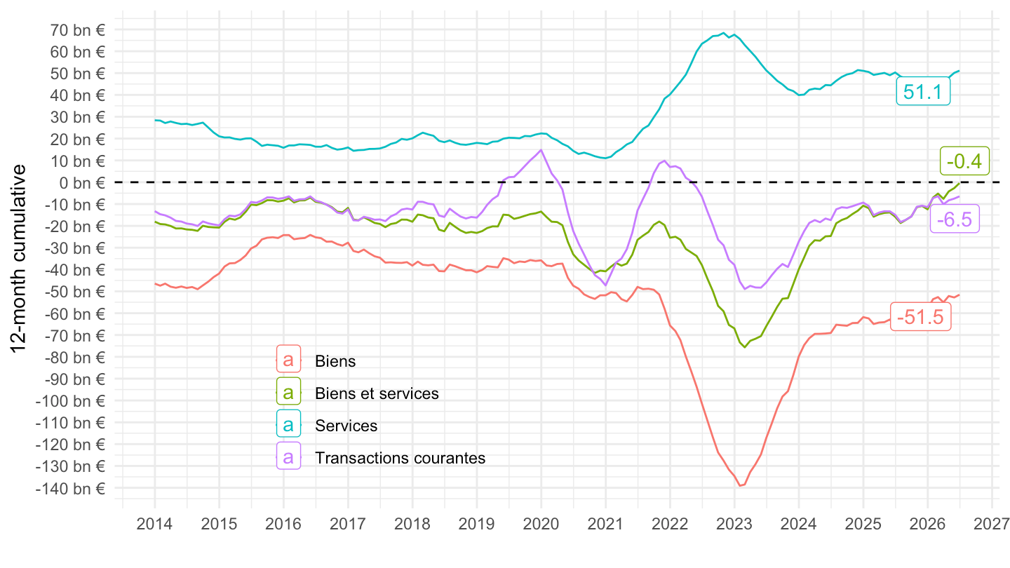
Services balance
BPM6.M.S.FR.W1.S1.S1.T.B.S._Z._Z._Z.EUR._T._X.N.ALL (Services) BPM6.M.S.FR.W1.S1.S1.T.B.SXD._Z._Z._Z.EUR._T._X.N.ALL (Services excluding travel) BPM6.M.S.FR.W1.S1.S1.T.B.SC._Z._Z._Z.EUR._T._X.N.ALL (Services - Transport) BPM6.M.N.FR.W1.S1.S1.T.D.SD._Z._Z._Z.EUR._T._X.N.ALL (Services, Travel)
12-month cumulative
Code
BPM6 |>

  # Services
  filter(variable == "BPM6.M.S.FR.W1.S1.S1.T.B.S._Z._Z._Z.EUR._T._X.N.ALL" |
           # Services excluding travel
         variable == "BPM6.M.S.FR.W1.S1.S1.T.B.SXD._Z._Z._Z.EUR._T._X.N.ALL" |
           # Services - Transport
         variable == "BPM6.M.S.FR.W1.S1.S1.T.B.SC._Z._Z._Z.EUR._T._X.N.ALL" |
           # Services, Travel
         variable == "BPM6.M.N.FR.W1.S1.S1.T.D.SD._Z._Z._Z.EUR._T._X.N.ALL") |>

  group_by(Int_acc_item) |>
  arrange(desc(date)) |>
  mutate(value = zoo::rollsum(value, 12, align = "left", fill = NA)) |>
  na.omit() |>
  ggplot() + geom_line(aes(x = date, y = value / 1000, color = Int_acc_item)) +

  theme_minimal() +
  scale_x_date(breaks = "1 year",
               labels = date_format("%Y")) +
  theme(legend.position = c(0.3, 0.8),
        legend.title = element_blank(),
        legend.direction = "vertical") +
  xlab("") + ylab("12-month cumulative") +
  scale_y_continuous(breaks = seq(-200, 200, 10),
                labels = dollar_format(suffix = " bn €",  accuracy = 1, prefix = "")) +
  geom_hline(yintercept = 0, linetype = "dashed") +
  geom_label_repel(data = . %>% filter(date == max(date)),
             aes(x = date, y = value/1000, color = Int_acc_item, label = round(value/1000, digits = 1)))
12-month cumulative
Code
BPM6 |>

  # Services
  filter(variable == "BPM6.M.S.FR.W1.S1.S1.T.B.S._Z._Z._Z.EUR._T._X.N.ALL" |
           # Services excluding travel
         variable == "BPM6.M.S.FR.W1.S1.S1.T.B.SXD._Z._Z._Z.EUR._T._X.N.ALL" |
           # Services, Travel
         variable == "BPM6.M.N.FR.W1.S1.S1.T.B.SD._Z._Z._Z.EUR._T._X.N.ALL") |>

  group_by(Int_acc_item) |>
  arrange(desc(date)) |>
  mutate(value = zoo::rollsum(value, 12, align = "left", fill = NA)) |>
  na.omit() |>
  ggplot() + geom_line(aes(x = date, y = value / 1000, color = Int_acc_item)) +

  theme_minimal() +
  scale_x_date(breaks = "1 year",
               labels = date_format("%Y")) +
  theme(legend.position = c(0.3, 0.8),
        legend.title = element_blank(),
        legend.direction = "vertical") +
  xlab("") + ylab("12-month cumulative") +
  scale_y_continuous(breaks = seq(-200, 200, 10),
                labels = dollar_format(suffix = " bn €",  accuracy = 1, prefix = "")) +
  geom_hline(yintercept = 0, linetype = "dashed") +
  geom_label_repel(data = . %>% filter(date == max(date)),
             aes(x = date, y = value/1000, color = Int_acc_item, label = round(value/1000, digits = 1)))
Goods balance (Customs vs. BPM6)
12-month cumulative
Code
BPM6 |>

  filter(variable == "BPM6.M.S.FR.W1.S1.S1.T.B.G1X._Z._Z._Z.EUR._T._X.N.ALL" |
         variable == "BPM6.M.S.FR.W1.S1.S1.T.B.G._Z._Z._Z.EUR._T._X.N.ALL" |
         variable == "BPM6.M.S.FR.W1.S1.S1.T.B.GX._Z._Z._Z.EUR._T._X.N.ALL") |>

  group_by(Int_acc_item) |>
  arrange(desc(date)) |>
  mutate(value = zoo::rollsum(value, 12, align = "left", fill = NA)) |>
  na.omit() |>
  ggplot() + geom_line(aes(x = date, y = value / 1000, color = Int_acc_item)) +

  theme_minimal() +
  scale_x_date(breaks = "1 year",
               labels = date_format("%Y")) +
  theme(legend.position = c(0.3, 0.2),
        legend.title = element_blank(),
        legend.direction = "vertical") +
  xlab("") + ylab("12-month cumulative") +
  scale_y_continuous(breaks = seq(-200, 200, 10),
                labels = dollar_format(suffix = " bn €",  accuracy = 1, prefix = "")) +
  geom_hline(yintercept = 0, linetype = "dashed") +
  geom_label_repel(data = . %>% filter(date == max(date)),
             aes(x = date, y = value/1000, color = Int_acc_item, label = round(value/1000, digits = 1)))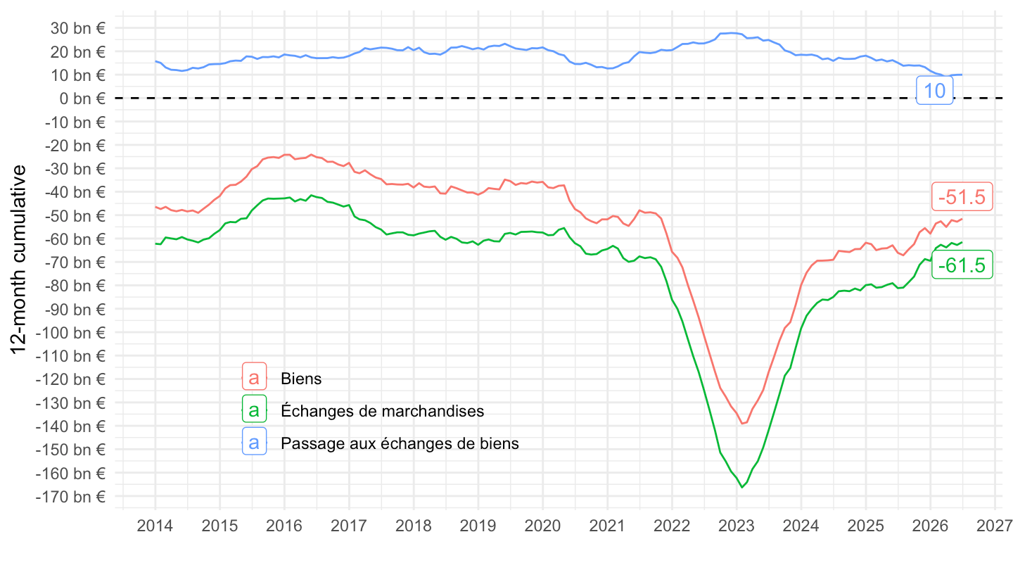
Balance - Services, Transport, Travel
Annual
Code
BPM6 |>

  filter(variable %in% c("BPM6.A.N.FR.W1.S1.S1.T.B.S._Z._Z._Z.EUR._T._X.N.ALL",
                         "BPM6.A.N.FR.W1.S1.S1.T.B.SD._Z._Z._Z.EUR._T._X.N.ALL",
                         "BPM6.A.N.FR.W1.S1.S1.T.B.SC._Z._Z._Z.EUR._T._X.N.ALL",
                         "BPM6.A.N.FR.W1.S1.S1.T.B.SXCD._Z._Z._Z.EUR._T._X.N.ALL")) |>

  left_join(gdp, by = "date") |>
  ggplot() + geom_line(aes(x = date, y = value/gdp / 1000, color = Int_acc_item)) +

  theme_minimal() +
  scale_x_date(breaks = "1 year",
               labels = date_format("%Y")) +
  theme(legend.position = c(0.3, 0.85),
        legend.title = element_blank(),
        legend.direction = "vertical",
        axis.text.x = element_text(angle = 45, vjust = 1, hjust = 1)) +
  xlab("") + ylab("Services balance (% of GDP)") +
  scale_y_continuous(breaks = 0.01*seq(-200, 200, .2),
                labels = percent_format(accuracy = .1),
                limits = 0.01*c(-0.6, 2.2)) +
  geom_hline(yintercept = 0, linetype = "dashed")
Quarterly
Code
BPM6 |>

  filter(variable %in% c("BPM6.Q.N.FR.W1.S1.S1.T.B.S._Z._Z._Z.EUR._T._X.N.ALL",
                         "BPM6.Q.N.FR.W1.S1.S1.T.B.SD._Z._Z._Z.EUR._T._X.N.ALL",
                         "BPM6.Q.N.FR.W1.S1.S1.T.B.SC._Z._Z._Z.EUR._T._X.N.ALL",
                         "BPM6.Q.N.FR.W1.S1.S1.T.B.SXCD._Z._Z._Z.EUR._T._X.N.ALL")) |>

  left_join(gdp_quarterly, by = "date") |>
  ggplot() + geom_line(aes(x = date, y = value/gdp / 1000, color = Int_acc_item)) +

  theme_minimal() +
  scale_x_date(breaks = "1 year",
               labels = date_format("%Y")) +
  theme(legend.position = c(0.2,0.9),
        legend.title = element_blank(),
        legend.direction = "vertical",
        axis.text.x = element_text(angle = 45, vjust = 1, hjust = 1)) +
  xlab("") + ylab("Services (Balance)") +
  scale_y_continuous(breaks = 0.01*seq(-200, 200, .2),
                labels = percent_format(accuracy = .1)) +
  geom_hline(yintercept = 0, linetype = "dashed")
Goods
Code
BPM6 |>

  filter(variable == "BPM6.A.N.FR.W1.S1.S1.T.C.G._Z._Z._Z.EUR._T._X.N.ALL" |
         variable == "BPM6.A.N.FR.W1.S1.S1.T.D.G._Z._Z._Z.EUR._T._X.N.ALL" |
         variable == "BPM6.A.N.FR.W1.S1.S1.T.B.G._Z._Z._Z.EUR._T._X.N.ALL") |>

  left_join(gdp, by = "date") |>
  ggplot() + geom_line(aes(x = date, y = value / gdp / 1000, color = Accounting_entry)) +

  theme_minimal() +
  scale_x_date(breaks = "1 year",
               labels = date_format("%Y")) +
  theme(legend.position = c(0.2,0.9),
        legend.title = element_blank(),
        legend.direction = "vertical",
        axis.text.x = element_text(angle = 45, vjust = 1, hjust = 1)) +
  xlab("") + ylab("Goods") +
  scale_y_continuous(breaks = 0.01*seq(-200, 200, 2),
                labels = percent_format(accuracy = 1))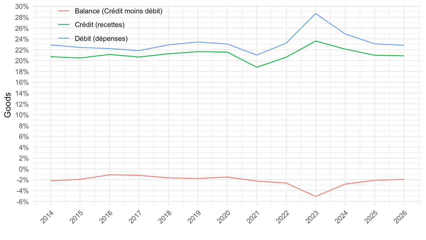
Services
Annual
Code
BPM6 |>

  filter(variable == "BPM6.A.N.FR.W1.S1.S1.T.C.S._Z._Z._Z.EUR._T._X.N.ALL" |
         variable == "BPM6.A.N.FR.W1.S1.S1.T.D.S._Z._Z._Z.EUR._T._X.N.ALL" |
         variable == "BPM6.A.N.FR.W1.S1.S1.T.B.S._Z._Z._Z.EUR._T._X.N.ALL") |>

  ggplot() + geom_line(aes(x = date, y = value / 1000, color = Accounting_entry)) +

  theme_minimal() +
  scale_x_date(breaks = "1 year",
               labels = date_format("%Y")) +
  theme(legend.position = c(0.2,0.9),
        legend.title = element_blank(),
        legend.direction = "vertical",
        axis.text.x = element_text(angle = 45, vjust = 1, hjust = 1)) +
  xlab("") + ylab("Travel Services") +
  scale_y_continuous(breaks = seq(-200, 2000, 20),
                labels = dollar_format(suffix = " bn €",  accuracy = 1, prefix = ""))
Quarterly
Code
BPM6 |>

  filter(variable == "BPM6.Q.N.FR.W1.S1.S1.T.C.SD._Z._Z._Z.EUR._T._X.N.ALL" |
         variable == "BPM6.Q.N.FR.W1.S1.S1.T.D.SD._Z._Z._Z.EUR._T._X.N.ALL" |
         variable == "BPM6.Q.N.FR.W1.S1.S1.T.B.SD._Z._Z._Z.EUR._T._X.N.ALL") |>

  ggplot() + geom_line(aes(x = date, y = value / 1000, color = Accounting_entry)) +

  theme_minimal() +
  scale_x_date(breaks = "1 year",
               labels = date_format("%Y")) +
  theme(legend.position = c(0.2,0.9),
        legend.title = element_blank(),
        legend.direction = "vertical",
        axis.text.x = element_text(angle = 45, vjust = 1, hjust = 1)) +
  xlab("") + ylab("") +
  scale_y_continuous(breaks = seq(-200, 200, 2),
                labels = dollar_format(suffix = " tn €",  accuracy = 1, prefix = ""))
Monthly
Code
BPM6 |>

  filter(variable == "BPM6.M.S.FR.W1.S1.S1.T.B.SD._Z._Z._Z.EUR._T._X.N.ALL" |
         variable == "BPM6.M.S.FR.W1.S1.S1.T.C.SD._Z._Z._Z.EUR._T._X.N.ALL" |
         variable == "BPM6.M.S.FR.W1.S1.S1.T.D.SD._Z._Z._Z.EUR._T._X.N.ALL") |>

  ggplot() + geom_line(aes(x = date, y = value / 1000, color = Accounting_entry)) +

  theme_minimal() +
  scale_x_date(breaks = "1 year",
               labels = date_format("%Y")) +
  theme(legend.position = c(0.2,0.9),
        legend.title = element_blank(),
        legend.direction = "vertical") +
  xlab("") + ylab("") +
  scale_y_continuous(breaks = seq(-200, 200, 2),
                labels = dollar_format(suffix = " tn €",  accuracy = 1, prefix = ""))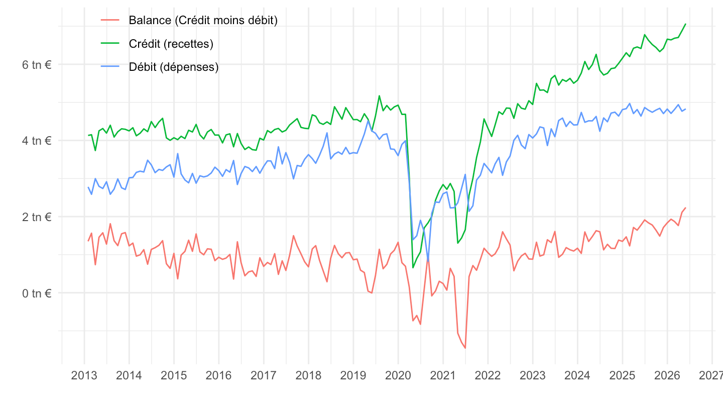
Transport Services
Annual
Code
BPM6 |>

  filter(variable == "BPM6.A.N.FR.W1.S1.S1.T.C.SC._Z._Z._Z.EUR._T._X.N.ALL" |
         variable == "BPM6.A.N.FR.W1.S1.S1.T.D.SC._Z._Z._Z.EUR._T._X.N.ALL" |
         variable == "BPM6.A.N.FR.W1.S1.S1.T.B.SC._Z._Z._Z.EUR._T._X.N.ALL") |>

  ggplot() + geom_line(aes(x = date, y = value / 1000, color = Accounting_entry)) +

  theme_minimal() +
  scale_x_date(breaks = "1 year",
               labels = date_format("%Y")) +
  theme(legend.position = c(0.2,0.9),
        legend.title = element_blank(),
        legend.direction = "vertical",
        axis.text.x = element_text(angle = 45, vjust = 1, hjust = 1)) +
  xlab("") + ylab("Travel Services") +
  scale_y_continuous(breaks = seq(-200, 200, 5),
                labels = dollar_format(suffix = " bn €",  accuracy = 1, prefix = ""))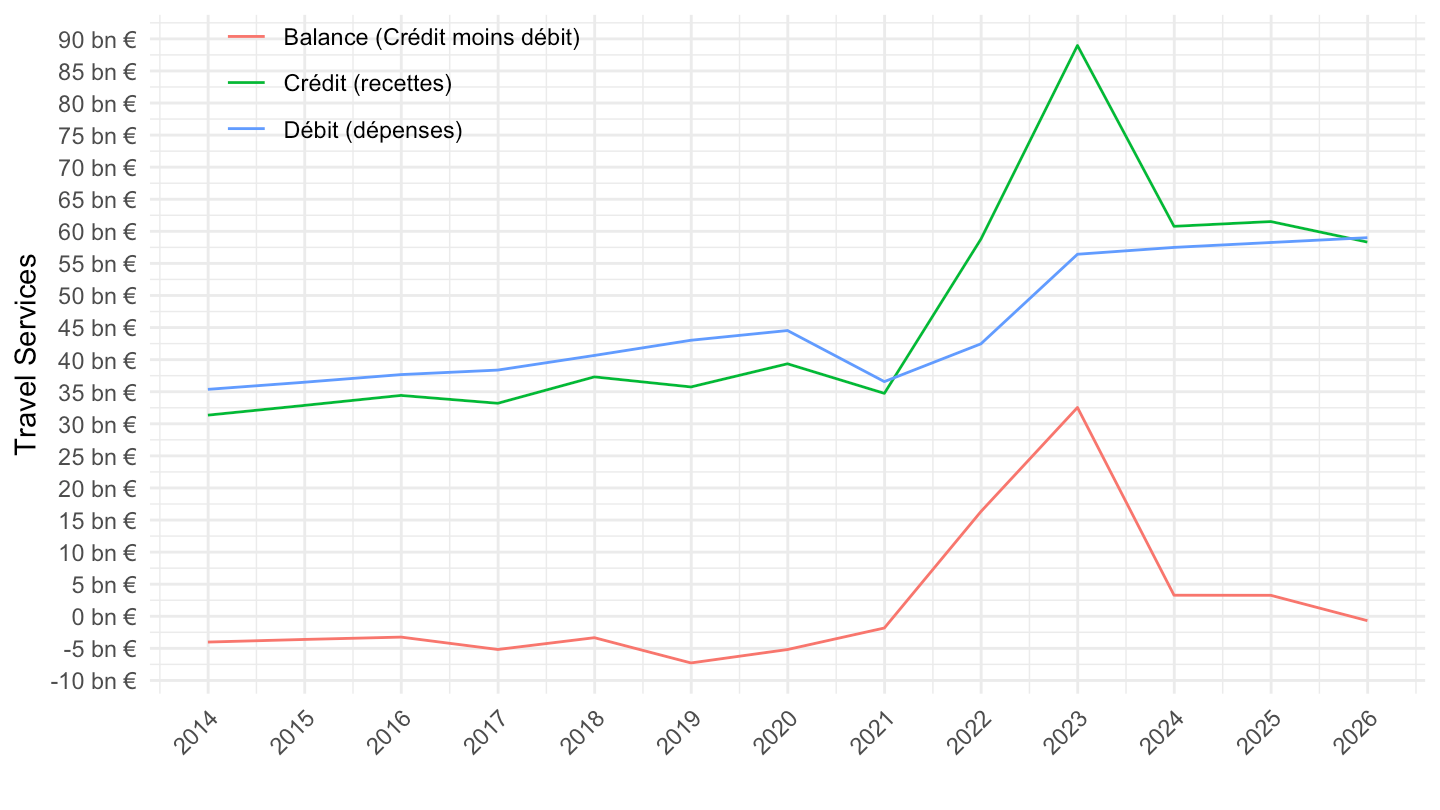
Quarterly
Code
BPM6 |>

  filter(variable == "BPM6.Q.N.FR.W1.S1.S1.T.C.SD._Z._Z._Z.EUR._T._X.N.ALL" |
         variable == "BPM6.Q.N.FR.W1.S1.S1.T.D.SD._Z._Z._Z.EUR._T._X.N.ALL" |
         variable == "BPM6.Q.N.FR.W1.S1.S1.T.B.SD._Z._Z._Z.EUR._T._X.N.ALL") |>

  ggplot() + geom_line(aes(x = date, y = value / 1000, color = Accounting_entry)) +

  theme_minimal() +
  scale_x_date(breaks = "1 year",
               labels = date_format("%Y")) +
  theme(legend.position = c(0.2,0.9),
        legend.title = element_blank(),
        legend.direction = "vertical",
        axis.text.x = element_text(angle = 45, vjust = 1, hjust = 1)) +
  xlab("") + ylab("") +
  scale_y_continuous(breaks = seq(-200, 200, 2),
                labels = dollar_format(suffix = " tn €",  accuracy = 1, prefix = ""))
Monthly
Code
BPM6 |>

  filter(variable == "BPM6.M.S.FR.W1.S1.S1.T.B.SD._Z._Z._Z.EUR._T._X.N.ALL" |
         variable == "BPM6.M.S.FR.W1.S1.S1.T.C.SD._Z._Z._Z.EUR._T._X.N.ALL" |
         variable == "BPM6.M.S.FR.W1.S1.S1.T.D.SD._Z._Z._Z.EUR._T._X.N.ALL") |>

  ggplot() + geom_line(aes(x = date, y = value / 1000, color = Accounting_entry)) +

  theme_minimal() +
  scale_x_date(breaks = "1 year",
               labels = date_format("%Y")) +
  theme(legend.position = c(0.2,0.9),
        legend.title = element_blank(),
        legend.direction = "vertical") +
  xlab("") + ylab("") +
  scale_y_continuous(breaks = seq(-200, 200, 2),
                labels = dollar_format(suffix = " tn €",  accuracy = 1, prefix = ""))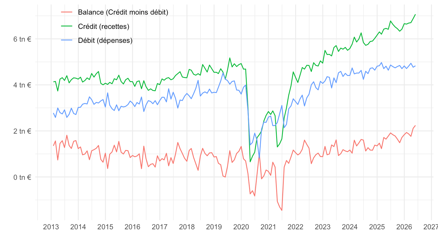
Travel Services
Annual
Code
BPM6 |>

  filter(variable == "BPM6.A.N.FR.W1.S1.S1.T.C.SD._Z._Z._Z.EUR._T._X.N.ALL" |
         variable == "BPM6.A.N.FR.W1.S1.S1.T.D.SD._Z._Z._Z.EUR._T._X.N.ALL" |
         variable == "BPM6.A.N.FR.W1.S1.S1.T.B.SD._Z._Z._Z.EUR._T._X.N.ALL") |>

  ggplot() + geom_line(aes(x = date, y = value / 1000, color = Accounting_entry)) +

  theme_minimal() +
  scale_x_date(breaks = "1 year",
               labels = date_format("%Y")) +
  theme(legend.position = c(0.2,0.9),
        legend.title = element_blank(),
        legend.direction = "vertical",
        axis.text.x = element_text(angle = 45, vjust = 1, hjust = 1)) +
  xlab("") + ylab("Travel Services") +
  scale_y_continuous(breaks = seq(-200, 200, 5),
                labels = dollar_format(suffix = " bn €",  accuracy = 1, prefix = ""))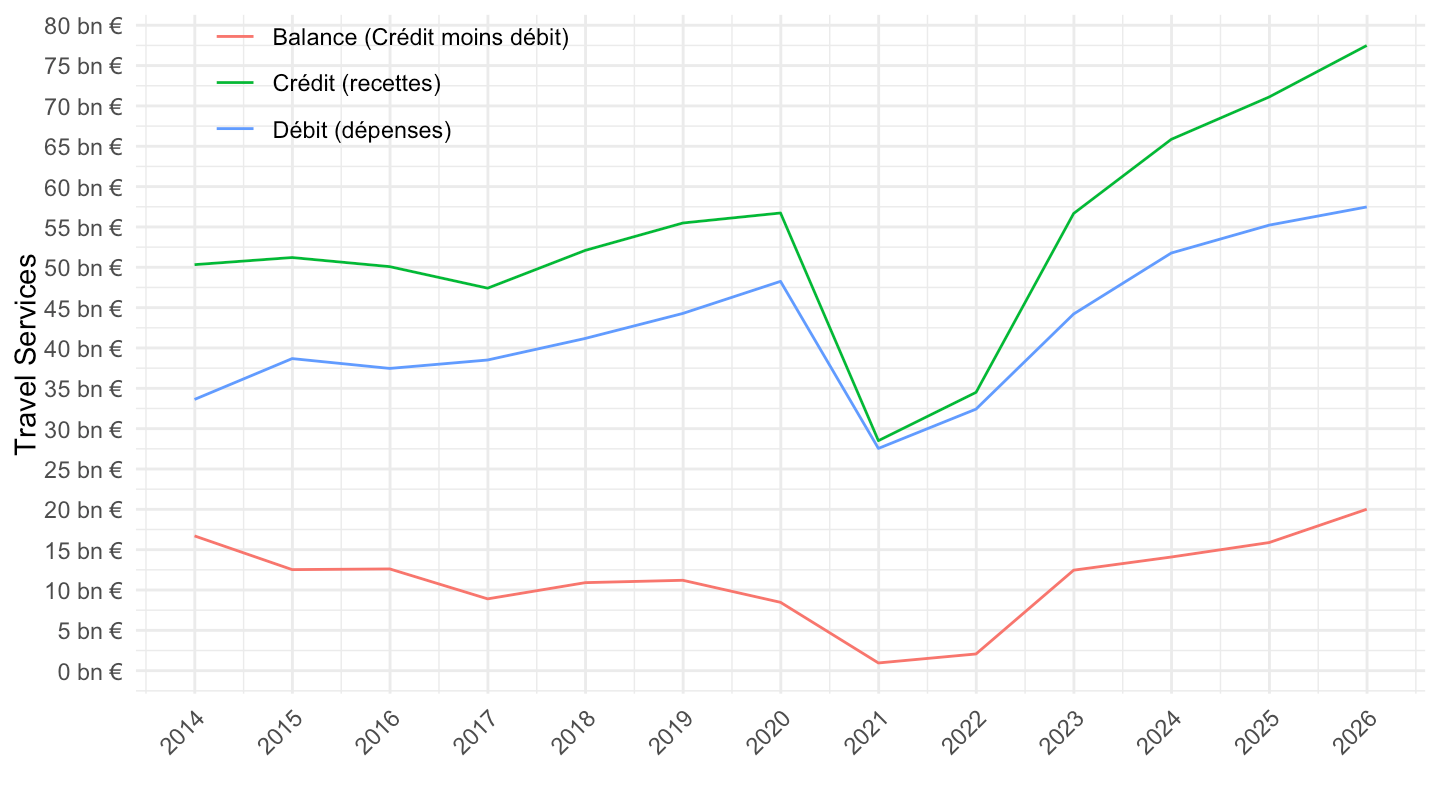
Quarterly
Code
BPM6 |>

  filter(variable == "BPM6.Q.N.FR.W1.S1.S1.T.C.SD._Z._Z._Z.EUR._T._X.N.ALL" |
         variable == "BPM6.Q.N.FR.W1.S1.S1.T.D.SD._Z._Z._Z.EUR._T._X.N.ALL" |
         variable == "BPM6.Q.N.FR.W1.S1.S1.T.B.SD._Z._Z._Z.EUR._T._X.N.ALL") |>

  ggplot() + geom_line(aes(x = date, y = value / 1000, color = Accounting_entry)) +

  theme_minimal() +
  scale_x_date(breaks = "1 year",
               labels = date_format("%Y")) +
  theme(legend.position = c(0.2,0.9),
        legend.title = element_blank(),
        legend.direction = "vertical",
        axis.text.x = element_text(angle = 45, vjust = 1, hjust = 1)) +
  xlab("") + ylab("") +
  scale_y_continuous(breaks = seq(-200, 200, 2),
                labels = dollar_format(suffix = " tn €",  accuracy = 1, prefix = ""))
Monthly
Code
BPM6 |>

  filter(variable == "BPM6.M.S.FR.W1.S1.S1.T.B.SD._Z._Z._Z.EUR._T._X.N.ALL" |
         variable == "BPM6.M.S.FR.W1.S1.S1.T.C.SD._Z._Z._Z.EUR._T._X.N.ALL" |
         variable == "BPM6.M.S.FR.W1.S1.S1.T.D.SD._Z._Z._Z.EUR._T._X.N.ALL") |>

  ggplot() + geom_line(aes(x = date, y = value / 1000, color = Accounting_entry)) +

  theme_minimal() +
  scale_x_date(breaks = "1 year",
               labels = date_format("%Y")) +
  theme(legend.position = c(0.2,0.9),
        legend.title = element_blank(),
        legend.direction = "vertical") +
  xlab("") + ylab("") +
  scale_y_continuous(breaks = seq(-200, 200, 1),
                labels = dollar_format(suffix = " tn €",  accuracy = 1, prefix = ""))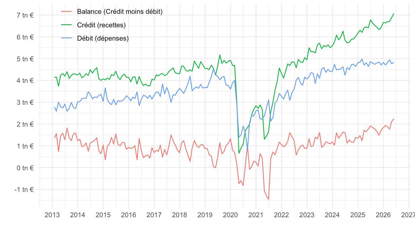
Portfolio investment
Quarterly
Code
BPM6 |>

  filter(variable == "BPM6.Q.N.FR.W1.S1.S1.T.A.FA.P.F._Z.EUR._T.M.N.ALL" |
         variable == "BPM6.Q.N.FR.W1.S1.S1.T.N.FA.P.F._Z.EUR._T.M.N.ALL") |>

  ggplot() + geom_line(aes(x = date, y = value / 1000, color = Variable)) +

  theme_minimal() +
  scale_x_date(breaks = "1 year",
               labels = date_format("%Y")) +
  theme(legend.position = c(0.3,0.1),
        legend.title = element_blank(),
        legend.direction = "vertical",
        axis.text.x = element_text(angle = 45, vjust = 1, hjust = 1)) +
  xlab("") + ylab("") +
  scale_y_continuous(breaks = seq(-200, 200, 20),
                labels = dollar_format(suffix = " tn €",  accuracy = 1, prefix = ""))
Primary Income
All
Code
BPM6 |>

  filter(variable == "BPM6.A.N.FR.W1.S1.S1.T.C.IN1._Z._Z._Z.EUR._T._X.N.ALL" |
         variable == "BPM6.A.N.FR.W1.S1.S1.T.D.IN1._Z._Z._Z.EUR._T._X.N.ALL" |
         variable == "BPM6.A.N.FR.W1.S1.S1.T.B.IN1._Z._Z._Z.EUR._T._X.N.ALL") |>

  ggplot() + geom_line(aes(x = date, y = value / 1000, color = Accounting_entry)) +

  theme_minimal() +
  scale_x_date(breaks = "2 years",
               labels = date_format("%Y")) +
  theme(legend.position = c(0.2,0.9),
        legend.title = element_blank(),
        legend.direction = "vertical") +
  xlab("") + ylab("Primary income") +
  scale_y_continuous(breaks = seq(-200, 1000, 20),
                labels = dollar_format(suffix = " bn €",  accuracy = 1, prefix = ""))
Portfolio
Code
BPM6 |>

  filter(variable == "BPM6.A.N.FR.W1.S1.S1.T.C.D4P.P.F._Z.EUR._T._X.N.ALL" |
         variable == "BPM6.A.N.FR.W1.S1.S1.T.B.D4P.P.F._Z.EUR._T._X.N.ALL" |
         variable == "BPM6.A.N.FR.W1.S1.S1.T.D.D4P.P.F._Z.EUR._T._X.N.ALL") |>

  ggplot() + geom_line(aes(x = date, y = value / 1000, color = Accounting_entry)) +

  theme_minimal() +
  scale_x_date(breaks = "1 year",
               labels = date_format("%Y")) +
  theme(legend.position = c(0.2,0.9),
        legend.title = element_blank(),
        legend.direction = "vertical",
        axis.text.x = element_text(angle = 45, vjust = 1, hjust = 1)) +
  xlab("") + ylab("Portfolio income") +
  scale_y_continuous(breaks = seq(-200, 1000, 20),
                labels = dollar_format(suffix = " bn €",  accuracy = 1, prefix = ""))
Other investment income
Code
BPM6 |>

  filter(variable == "BPM6.A.N.FR.W1.S1.S1.T.C.D4P.O.F._Z.EUR._T._X.N.ALL" |
         variable == "BPM6.A.N.FR.W1.S1.S1.T.D.D4P.O.F._Z.EUR._T._X.N.ALL" |
         variable == "BPM6.A.N.FR.W1.S1.S1.T.B.D4P.O.F._Z.EUR._T._X.N.ALL") |>

  ggplot() + geom_line(aes(x = date, y = value / 1000, color = Accounting_entry)) +

  theme_minimal() +
  scale_x_date(breaks = "1 year",
               labels = date_format("%Y")) +
  theme(legend.position = c(0.2,0.9),
        legend.title = element_blank(),
        legend.direction = "vertical",
        axis.text.x = element_text(angle = 45, vjust = 1, hjust = 1)) +
  xlab("") + ylab("Portfolio income") +
  scale_y_continuous(breaks = seq(-200, 1000, 10),
                labels = dollar_format(suffix = " bn €",  accuracy = 1, prefix = ""))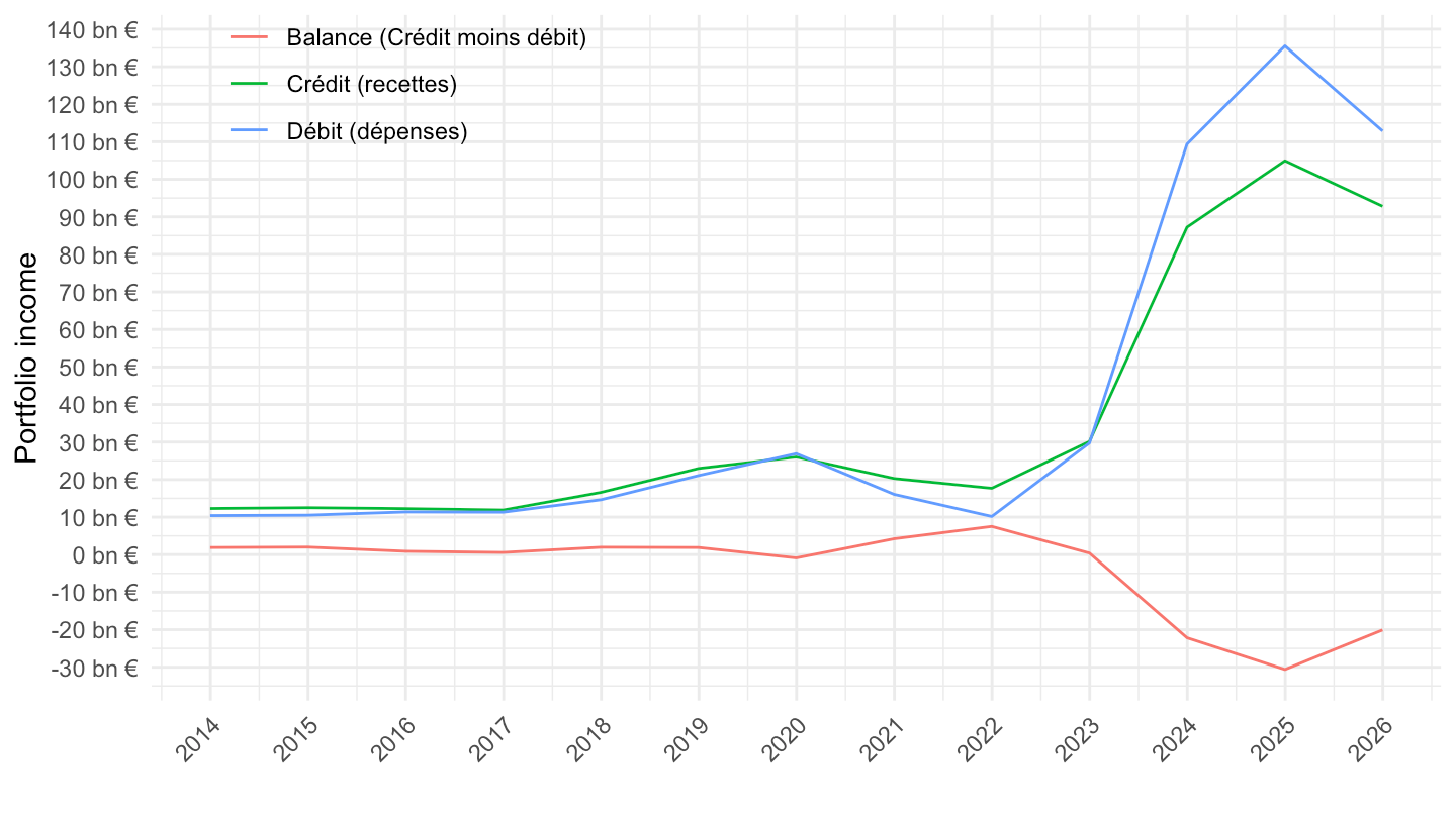
Investment income
Code
BPM6 |>

  filter(variable == "BPM6.A.N.FR.W1.S1.S1.T.B.D4P._T.F._Z.EUR._T._X.N.ALL" |
         variable == "BPM6.A.N.FR.W1.S1.S1.T.C.D4P._T.F._Z.EUR._T._X.N.ALL" |
         variable == "BPM6.A.N.FR.W1.S1.S1.T.D.D4P._T.F._Z.EUR._T._X.N.ALL") |>

  ggplot() + geom_line(aes(x = date, y = value / 1000, color = Accounting_entry)) +

  theme_minimal() +
  scale_x_date(breaks = "1 year",
               labels = date_format("%Y")) +
  theme(legend.position = c(0.2,0.9),
        legend.title = element_blank(),
        legend.direction = "vertical",
        axis.text.x = element_text(angle = 45, vjust = 1, hjust = 1)) +
  xlab("") + ylab("Investment income") +
  scale_y_continuous(breaks = seq(-200, 1000, 20),
                labels = dollar_format(suffix = " bn €",  accuracy = 1, prefix = ""))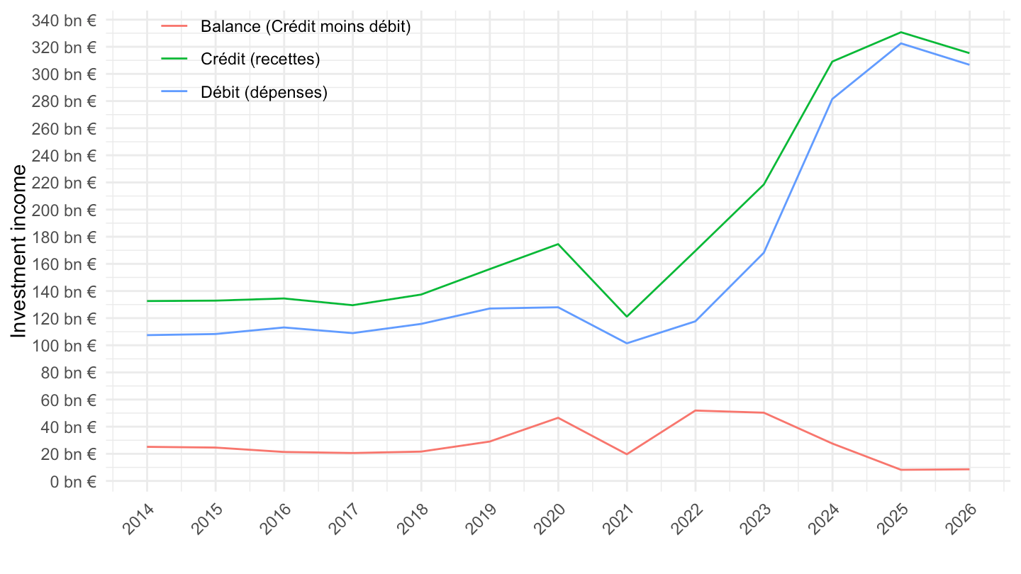
Direct investment income
Code
BPM6 |>

  filter(variable == "BPM6.A.N.FR.W1.S1.S1.T.B.D4P.D.F._Z.EUR._T._X.N.ALL" |
         variable == "BPM6.A.N.FR.W1.S1.S1.T.C.D4P.D.F._Z.EUR._T._X.N.ALL" |
         variable == "BPM6.A.N.FR.W1.S1.S1.T.D.D4P.D.F._Z.EUR._T._X.N.ALL") |>

  ggplot() + geom_line(aes(x = date, y = value / 1000, color = Accounting_entry)) +

  theme_minimal() +
  scale_x_date(breaks = "1 year",
               labels = date_format("%Y")) +
  theme(legend.position = c(0.2,0.9),
        legend.title = element_blank(),
        legend.direction = "vertical",
        axis.text.x = element_text(angle = 45, vjust = 1, hjust = 1)) +
  xlab("") + ylab("Direct investment income") +
  scale_y_continuous(breaks = seq(-200, 1000, 10),
                labels = dollar_format(suffix = " bn €",  accuracy = 1, prefix = ""))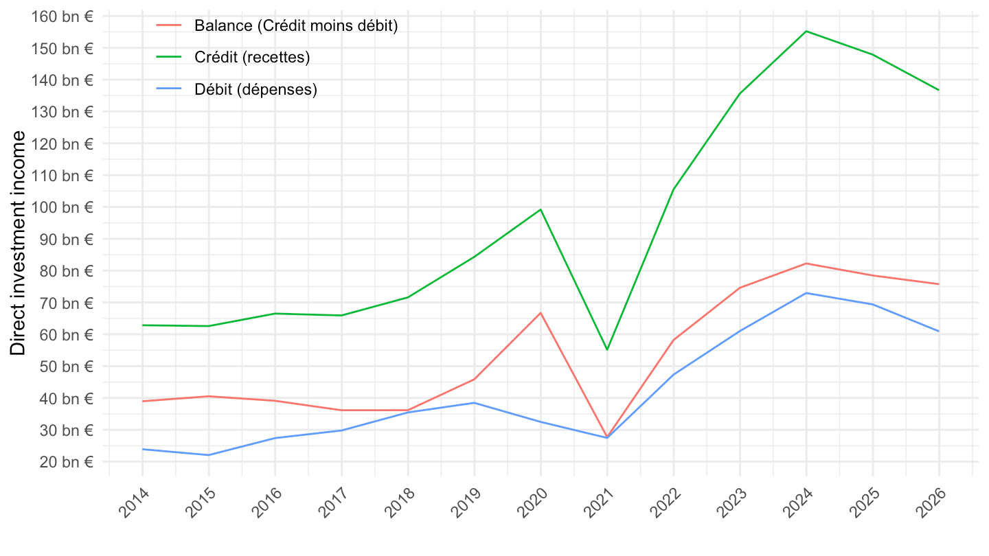
Balance
Code
BPM6 |>

  filter(variable == "BPM6.A.N.FR.W1.S1.S1.T.B.D4P.D.F._Z.EUR._T._X.N.ALL" |
         variable == "BPM6.A.N.FR.W1.S1.S1.T.B.D4P._T.F._Z.EUR._T._X.N.ALL" |
         variable == "BPM6.A.N.FR.W1.S1.S1.T.B.D4P.O.F._Z.EUR._T._X.N.ALL" |
         variable == "BPM6.A.N.FR.W1.S1.S1.T.B.D4P.P.F._Z.EUR._T._X.N.ALL") |>

  ggplot() + geom_line(aes(x = date, y = value / 1000, color = Functional_cat)) +

  theme_minimal() + xlab("") + ylab("Primary income") +
  scale_x_date(breaks = "1 year",
               labels = date_format("%Y")) +
  theme(legend.position = c(0.25, 0.85),
        legend.title = element_blank(),
        legend.direction = "vertical",
        axis.text.x = element_text(angle = 45, vjust = 1, hjust = 1)) +
  scale_y_continuous(breaks = seq(-200, 1000, 10),
                labels = dollar_format(suffix = " bn €",  accuracy = 1, prefix = ""))
Balance
Code
BPM6 |>

  filter(grepl("BPM6.A.N.FR.W1.S1.S1.T.B.D4P.", variable)) |>

  ggplot() + geom_line(aes(x = date, y = value / 1000, color = Functional_cat)) +

  theme_minimal() + xlab("") + ylab("Primary income") +
  scale_x_date(breaks = "1 year",
               labels = date_format("%Y")) +
  theme(legend.position = c(0.25, 0.85),
        legend.title = element_blank(),
        legend.direction = "vertical",
        axis.text.x = element_text(angle = 45, vjust = 1, hjust = 1)) +
  scale_y_continuous(breaks = seq(-200, 1000, 10),
                labels = dollar_format(suffix = " bn €",  accuracy = 1, prefix = ""))
Secondary Income
All
Code
BPM6 |>

  filter(grepl("BPM6.A.N.FR.W1.S1.S1.T.B.IN2.", variable) |
         grepl("BPM6.A.N.FR.W1.S1.S1.T.C.IN2.", variable) |
         grepl("BPM6.A.N.FR.W1.S1.S1.T.D.IN2.", variable)) |>

  ggplot() + geom_line(aes(x = date, y = value / 1000, color = Accounting_entry)) +

  theme_minimal() + xlab("") + ylab("Secondary income") +
  scale_x_date(breaks = "1 year",
               labels = date_format("%Y")) +
  theme(legend.position = c(0.25, 0.85),
        legend.title = element_blank(),
        legend.direction = "vertical",
        axis.text.x = element_text(angle = 45, vjust = 1, hjust = 1)) +
  scale_y_continuous(breaks = seq(-200, 1000, 10),
                labels = dollar_format(suffix = " bn €",  accuracy = 1, prefix = ""))
Balance
Code
BPM6 |>

  filter(grepl("BPM6.A.N.FR.W1.S1.S1.T.B.IN2.", variable)) |>

  ggplot() + geom_line(aes(x = date, y = value / 1000, color = Functional_cat)) +

  theme_minimal() + xlab("") + ylab("Secondary income") +
  scale_x_date(breaks = "1 year",
               labels = date_format("%Y")) +
  theme(legend.position = c(0.25, 0.85),
        legend.title = element_blank(),
        legend.direction = "vertical",
        axis.text.x = element_text(angle = 45, vjust = 1, hjust = 1)) +
  scale_y_continuous(breaks = seq(-200, 1000, 2),
                labels = dollar_format(suffix = " bn €",  accuracy = 1, prefix = ""))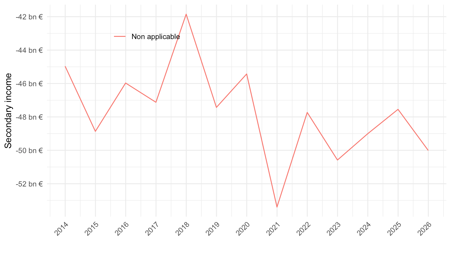
Current Account
All
Code
BPM6 |>

  filter(FREQ == "M",
         INT_ACC_ITEM %in% c("G", "S", "G1X"),
         ADJUSTMENT == "S",
         REF_SECTOR == "S1",
         COUNTERPART_SECTOR == "S1",
         FLOW_STOCK_ENTRY == "T",
         ACCOUNTING_ENTRY == "B") |>

  ggplot() + geom_line(aes(x = date, y = value / 1000, color = Int_acc_item)) +

  theme_minimal() +
  scale_x_date(breaks = "1 year",
               labels = date_format("%Y")) +
  theme(legend.position = c(0.3,0.1),
        legend.title = element_blank(),
        legend.direction = "vertical") +
  xlab("") + ylab("") +
  scale_y_continuous(breaks = seq(-100, 10, 1),
                labels = dollar_format(suffix = " tn €",  accuracy = 1, prefix = ""))
2018-
Code
BPM6 |>

  filter(date >= as.Date("2018-01-01"),
         FREQ == "M",
         ADJUSTMENT == "S",
         COUNTERPART_AREA == "W1",
         REF_SECTOR == "S1",
         COUNTERPART_SECTOR == "S1",
         FLOW_STOCK_ENTRY == "T",
         ACCOUNTING_ENTRY == "B",
         INT_ACC_ITEM %in% c("G", "S")) |>

  ggplot() + geom_line(aes(x = date, y = value / 1000, color = Int_acc_item)) +

  theme_minimal() + xlab("") + ylab("") +
  scale_x_date(breaks = "3 months",
               labels = date_format("%b-%Y")) +
  theme(legend.position = c(0.3,0.1),
        legend.title = element_blank(),
        legend.direction = "vertical",
        axis.text.x = element_text(angle = 45, vjust = 1, hjust = 1)) +
  scale_y_continuous(breaks = seq(-100, 10, 1),
                labels = dollar_format(suffix = " tn €",  accuracy = 1, prefix = ""))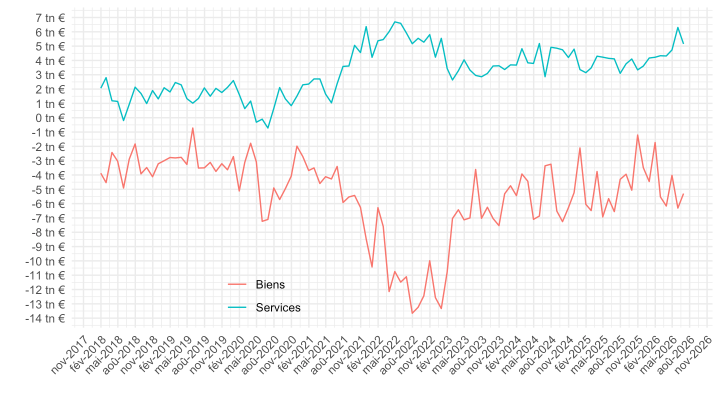
Table - Monthly
Code
BPM6 |>

  filter(date == as.Date("2018-01-01"),
         FREQ == "M",
         ADJUSTMENT == "S",
         REF_SECTOR == "S1",
         COUNTERPART_SECTOR == "S1",
         FLOW_STOCK_ENTRY == "T",
         ACCOUNTING_ENTRY == "B") |>


  select(Int_acc_item, Functional_cat, value) |>
print_table_conditional()| Int_acc_item | Functional_cat | value |
|---|---|---|
| NA | NA | NA |
| :------------: | :--------------: | :-----: |
France vis-à-vis Germany
All
Code
BPM6 |>

  filter(FREQ == "A",
         COUNTERPART_AREA == "DE",
         ACCOUNTING_ENTRY == "B",
         INT_ACC_ITEM %in% c("G", "S")) |>

  ggplot() + geom_line(aes(x = date, y = value / 1000, color = Int_acc_item)) +

  theme_minimal() +  xlab("") + ylab("") +
  scale_x_date(breaks = "1 year",
               labels = date_format("%Y")) +
  theme(legend.position = c(0.3,0.1),
        legend.title = element_blank(),
        legend.direction = "vertical") +
  scale_y_continuous(breaks = seq(-40, 10, 1),
                labels = dollar_format(suffix = " bn €",  accuracy = 1, prefix = ""))
Goods
Code
COUNTERPART_AREA <- read_parquet("COUNTERPART_AREA.parquet")
BPM6 |>

  filter(FREQ == "A",
         COUNTERPART_AREA %in% c("DE", "CN"),
         ACCOUNTING_ENTRY == "B",
         INT_ACC_ITEM %in% c("G")) |>

  left_join(colors, by = c("Counterpart_area" = "country")) |>
  mutate(value = value / 1000) |>
  mutate(Ref_area = Counterpart_area) |>
  ggplot() + geom_line(aes(x = date, y = value, color = color)) +
  scale_color_identity() + add_2flags +
  theme_minimal() +  xlab("") + ylab("") +
  scale_x_date(breaks = "1 year",
               labels = date_format("%Y")) +
  theme(legend.position = c(0.3,0.1),
        legend.title = element_blank(),
        legend.direction = "vertical") +
  scale_y_continuous(breaks = seq(-100, 10, 5),
                labels = dollar_format(suffix = " bn €",  accuracy = 1, prefix = ""))
Services
Code
COUNTERPART_AREA <- read_parquet("COUNTERPART_AREA.parquet")
BPM6 |>

  filter(FREQ == "A",
         COUNTERPART_AREA %in% c("DE", "CN"),
         ACCOUNTING_ENTRY == "B",
         INT_ACC_ITEM %in% c("S")) |>

  left_join(colors, by = c("Counterpart_area" = "country")) |>
  mutate(value = value / 1000) |>
  mutate(Ref_area = Counterpart_area) |>
  ggplot() + geom_line(aes(x = date, y = value, color = color)) +
  scale_color_identity() + add_2flags +
  theme_minimal() +  xlab("") + ylab("") +
  scale_x_date(breaks = "1 year",
               labels = date_format("%Y")) +
  theme(legend.position = c(0.3,0.1),
        legend.title = element_blank(),
        legend.direction = "vertical") +
  scale_y_continuous(breaks = seq(-40, 10, 1),
                labels = dollar_format(suffix = " bn €",  accuracy = 1, prefix = ""))
Goods and Services
Code
COUNTERPART_AREA <- read_parquet("COUNTERPART_AREA.parquet")
BPM6 |>

  filter(FREQ == "A",
         COUNTERPART_AREA %in% c("DE", "CN"),
         ACCOUNTING_ENTRY == "B",
         INT_ACC_ITEM %in% c("S", "G")) %>%
  select_if(~ n_distinct(.) > 1) |>
  group_by(date, COUNTERPART_AREA) |>
  summarise(value = sum(value)) |>
  left_join(COUNTERPART_AREA, by = "COUNTERPART_AREA") |>
  left_join(colors, by = c("Counterpart_area" = "country")) |>
  mutate(value = value / 1000) |>
  mutate(Ref_area = Counterpart_area) |>
  ggplot() + geom_line(aes(x = date, y = value, color = color)) +
  scale_color_identity() + add_2flags +
  theme_minimal() +  xlab("") + ylab("Bilateral deficit with France (Source: Banque de France)") +
  scale_x_date(breaks = "1 year",
               labels = date_format("%Y")) +
  theme(legend.position = c(0.3,0.1),
        legend.title = element_blank(),
        legend.direction = "vertical") +
  scale_y_continuous(breaks = seq(-40, 10, 2),
                labels = dollar_format(suffix = " bn €",  accuracy = 1, prefix = ""))
France vis-à-vis China
All
Quarterly
Code
BPM6 |>

  filter(FREQ == "A",
         COUNTERPART_AREA == "CN",
         ACCOUNTING_ENTRY == "B",
         INT_ACC_ITEM %in% c("G", "S")) |>

  ggplot() + geom_line(aes(x = date, y = value / 1000, color = Int_acc_item)) +

  theme_minimal() +
  scale_x_date(breaks = "1 year",
               labels = date_format("%Y")) +
  theme(legend.position = c(0.3,0.1),
        legend.title = element_blank(),
        legend.direction = "vertical") +
  xlab("") + ylab("") +
  scale_y_continuous(breaks = seq(-100, 10, 5),
                labels = dollar_format(suffix = " bn €",  accuracy = 1, prefix = ""))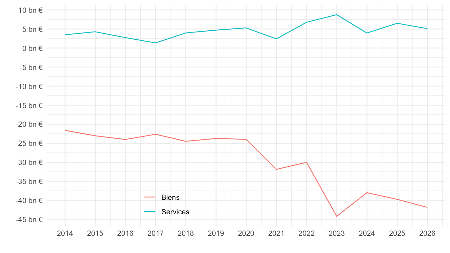
Quarterly
Code
BPM6 |>

  filter(FREQ == "A",
         INT_ACC_ITEM %in% c("G", "S", "G1X"),
         COUNTERPART_AREA == "CN",
         REF_SECTOR == "S1",
         COUNTERPART_SECTOR == "S1",
         FLOW_STOCK_ENTRY == "T",
         ACCOUNTING_ENTRY == "B",
         INT_ACC_ITEM %in% c("G", "S")) |>

  ggplot() + geom_line(aes(x = date, y = value / 1000, color = Int_acc_item)) +

  theme_minimal() +
  scale_x_date(breaks = "1 year",
               labels = date_format("%Y")) +
  theme(legend.position = c(0.3, 0.1),
        legend.title = element_blank(),
        legend.direction = "vertical") +
  xlab("") + ylab("") +
  scale_y_continuous(breaks = seq(-50, 10, 5),
                labels = dollar_format(suffix = " bn €",  accuracy = 1, prefix = ""))
Table
Code
BPM6 |>

  filter(date == as.Date("2020-03-31"),
         FREQ == "Q",
         INT_ACC_ITEM %in% c("G"),
         REF_SECTOR == "S1",
         COUNTERPART_SECTOR == "S1",
         FLOW_STOCK_ENTRY == "T",
         ACCOUNTING_ENTRY == "B") |>
  select(COUNTERPART_AREA, Variable, value) |>
print_table_conditional()| COUNTERPART_AREA | Variable | value |
|---|---|---|
| J9 | Transactions courantes - Biens - Ensemble de l'économie - Solde - France vis-à-vis hors Zone Euro - Brut | -6778 |
| JP | Transactions courantes - Biens - Ensemble de l'économie - Solde - France vis-à-vis Japon - Brut | -938 |
| W1 | Transactions courantes - Biens - Ensemble de l'économie - Solde - France vis-à-vis Reste du monde - Brut | -13919 |
| B6 | Transactions courantes - Biens - Ensemble de l'économie - Solde - France vis-à-vis de l'Union européenne (27 membres) - Trimestriel - Brut | -7510 |
| CH | Transactions courantes - Biens - Ensemble de l'économie - Solde - France vis-à-vis Suisse - Brut | 798 |
| I9 | Transactions courantes - Biens - Ensemble de l'économie - Solde - France vis-à-vis Zone Euro - Brut | -7142 |
| CN | Transactions courantes - Biens - Ensemble de l'économie - Solde - France vis-à-vis Chine - Brut | -8069 |
| Q6 | Transactions courantes - Biens - Ensemble de l'économie - Solde -France vis-à-vis de l'Union européenne à 28, hors zone euro à 18, à l?exclusion du Royaume-Uni, du Danemark et de la Suède - Brut | -416 |
| US | Transactions courantes - Biens - Ensemble de l'économie - Solde - France vis-à-vis États Unis - Brut | 651 |
Goods
Code
BPM6 |>

  filter(date >= as.Date("2016-12-31"),
         FREQ == "Q",
         INT_ACC_ITEM %in% c("G"),
         REF_SECTOR == "S1",
         COUNTERPART_AREA %in% c("W1", "I8", "J8"),
         COUNTERPART_SECTOR == "S1",
         FLOW_STOCK_ENTRY == "T",
         ACCOUNTING_ENTRY == "B") |>

  ggplot() + geom_line(aes(x = date, y = value / 1000, color = Counterpart_area)) +

  theme_minimal() + xlab("") + ylab("") +
  scale_x_date(breaks = "1 year",
               labels = date_format("%Y")) +
  theme(legend.position = c(0.6, 0.1),
        legend.title = element_blank(),
        legend.direction = "vertical") +
  scale_y_continuous(breaks = seq(-30, 30, 2),
                labels = dollar_format(suffix = " tn €",  accuracy = 1, prefix = ""))
2010
Code
BPM6 |>

  filter(date >= as.Date("2010-12-31"),
         FREQ == "Q",
         INT_ACC_ITEM %in% c("G"),
         REF_SECTOR == "S1",
         COUNTERPART_AREA %in% c("W1", "I8", "J8"),
         COUNTERPART_SECTOR == "S1",
         FLOW_STOCK_ENTRY == "T",
         ACCOUNTING_ENTRY == "B") |>

  ggplot() + geom_line(aes(x = date, y = value / 1000, color = Counterpart_area)) +

  theme_minimal() + xlab("") + ylab("") +
  scale_x_date(breaks = "1 year",
               labels = date_format("%Y")) +
  theme(legend.position = c(0.6, 0.1),
        legend.title = element_blank(),
        legend.direction = "vertical") +
  scale_y_continuous(breaks = seq(-30, 30, 2),
                labels = dollar_format(suffix = " tn €",  accuracy = 1, prefix = ""))
Net External Debt
Code
BPM6 |>

  filter(variable %in% c("BPM6.A.N.FR.W1.S1.S1.LE.N.FA._T.FNED._Z.PCPIB._T._X.N.ALL",
                         "BPM6.A.N.FR.W1.S1.S1.LE.N.FA._T.F._Z.PCPIB._T._X.N.ALL")) |>
  ggplot() + geom_line(aes(x = date, y = value/100, color = Variable)) +
  xlab("") + ylab("") + theme_minimal() +

  scale_x_date(breaks = "2 years",
               labels = date_format("%Y")) +
  scale_y_continuous(breaks = 0.01*seq(-200, 140, 10),
                labels = percent_format(accuracy = 1)) +
  theme(legend.position = c(0.3, 0.9),
        legend.title = element_blank(),
        legend.direction = "vertical")