Investment

ENPC, 2nd year - SEGF

François Geerolf

OFCE/Sciences Po, CEPR

Current-Cost Net Stock of Fixed Assets and Consumer Durable Goods

What is capital ?

What is capital ?

Fixed Assets and consumer durables

Pourquoi un taux d’actualisation?

Intuition de base

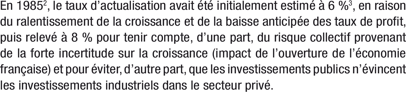
• Les investissements publics ne doivent pas évincer les investissements privés.

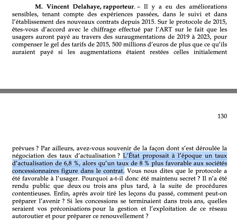
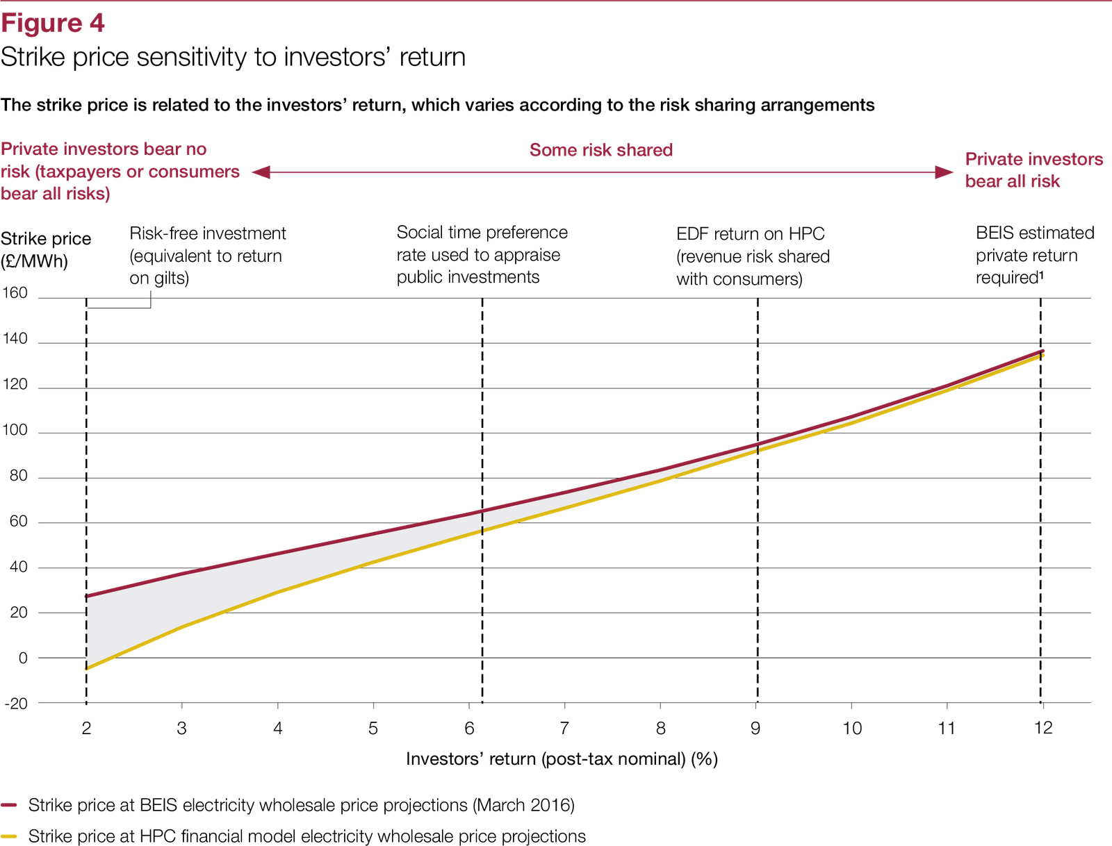
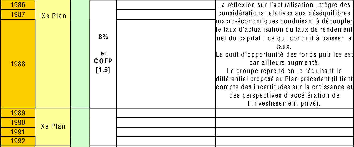
• Si le privé est capable d’obtenir des rendements de 8%, alors il n’y a pas de raison que le public ne s’impose pas le même taux d’actualisation.

• Comme le taux d’actualisation “de base” parait trop élevé, on a dit que les marchés étaient “trop court-termistes”, et qu’il fallait à sa place utiliser un taux d’actualisation plus faible.

Taux de marchés VS taux d’actualisation social

• Ce taux d’actualisation est souvent fondé sur la règle de Ramsey:

\[\boxed{r=\delta + \gamma g}\]

• Cependant: hypothèese de stagnation séculaire = les rendements sur les investissements risqués sont également bas. En réalité, il n’y a pas vraiment de rareté des capitaux, bien au contraire.

• Si on pense que le taux d’actualisation est \(r=g\) alors on veut réaliser davantage d’investissements publics, ou en tout cas les évaluer à partir d’une règle de taux d’intérêt qui est bien plus faible.

Souci: Eviction de l’investissement privé

Source: Rapport Gollier (2011). pdf

Senat 2020

Impact de r sur valeur du carbone

Energie nucléaire

Vision anglo-saxonne

Vente des autoroutes: Villepin

Utilisation de la prime de risque

Points importants

• Etat faible lorsqu’il négocie de gré à gré.

• Appel d’offres ouvert et compétitif (18 candidats).

• Moyen plus efficace pour obtenir le meilleur prix.

Points importants

• Les intérêts de l’Etat ont-ils été bien préservés.

• Garantir un juste prix.

• Cours de bourse ? 10 à 12 milliards d’euros.

• Rapport cour des comptes: 24 milliards d’€. (14.8 milliards)

Commission participations et transferts

• Bradé les bijoux de famille.

• Tué la poule aux oeufs d’or.

• L’APE a conservé

• Procédure a eu lieu en 2 temps.

• Un des lots: celui à Vinci, il n’y avait qu’un seul concurrent. (moins élevé par rapport au prix minimum versé)

Appel d’offres

• On est dans un appel d’offres.

• Procédure.

• Commission Nationale des Participations et des Transferts.

• Le pouvoir politique n’a pas le moyen d’entrer dans ce débat.

Historique des taux utilisés

Quelques jalons

• Logique très saine: hiérarchiser les projets d’investissement en fonction de leur intérêt socioéconomique.

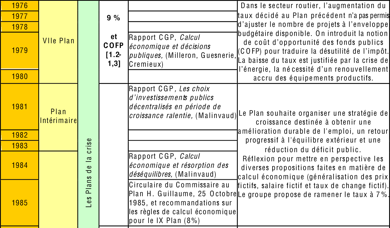
• 1994: Rapport Boiteux.

• 2005: Rapport Lebesgue.

• 2011: Rapport Gollier.

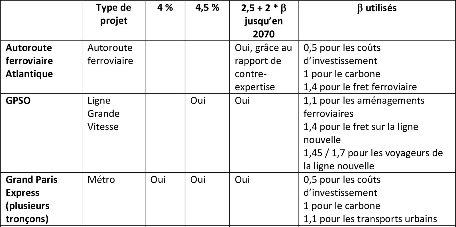
• 2013: Commission Quinet: Taux de 2.5% + Prime de Risque de 2%.

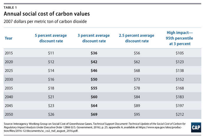
• Une manière de favoriser l’investissement, tout en restant dans une logique de rationalisation de la dépense publique, serait simplement de diminuer le taux d’actualisation.

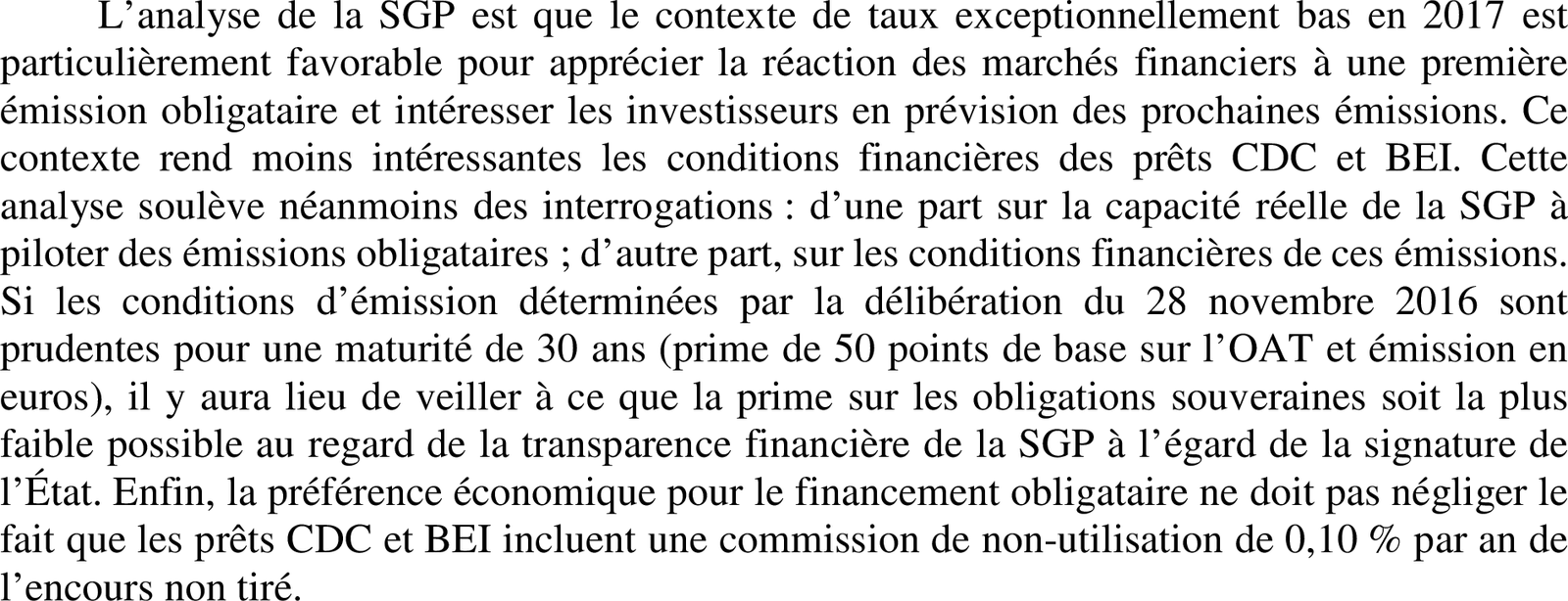
• Cela a été fait indirectement par la SGP, dont les frais financiers correspondent à des taux d’intérêt très bas.

1985

Rapport Lebesgue (2005)

• Rapport Lebègue (2005) a repris la base théorique utilisée par le Trésor britannique

• Importance de la croissance française anticipée.

• Préconise un taux d’actualisation sans risque de 4 % jusqu’à trente ans et décroissant jusqu’à 2 % au-delà.

• Taux de 4 % (\(\alpha\) = 1 % + 2*1,5 %) est obtenu en retenant un taux de préférence pure pour le présent \(\delta = 1\) %, une élasticité de l’utilité marginale de la consommation \(\gamma = 2\) et une croissance économique de référence μ = 1,5 %.

• La décroissance proposée est obtenue en prenant une prévision de croissance économique par tête qui peut varier entre deux extrêmes, 2 % avec une probabilité de 2/3 et 0,5 % avec une probabilité de 1/3.

Rapport Gollier (2011)

Rapport Gollier (2011)

Commission Quinet (2013)

• Taux d’actualisation français fixé par la Commission Quinet (2013).

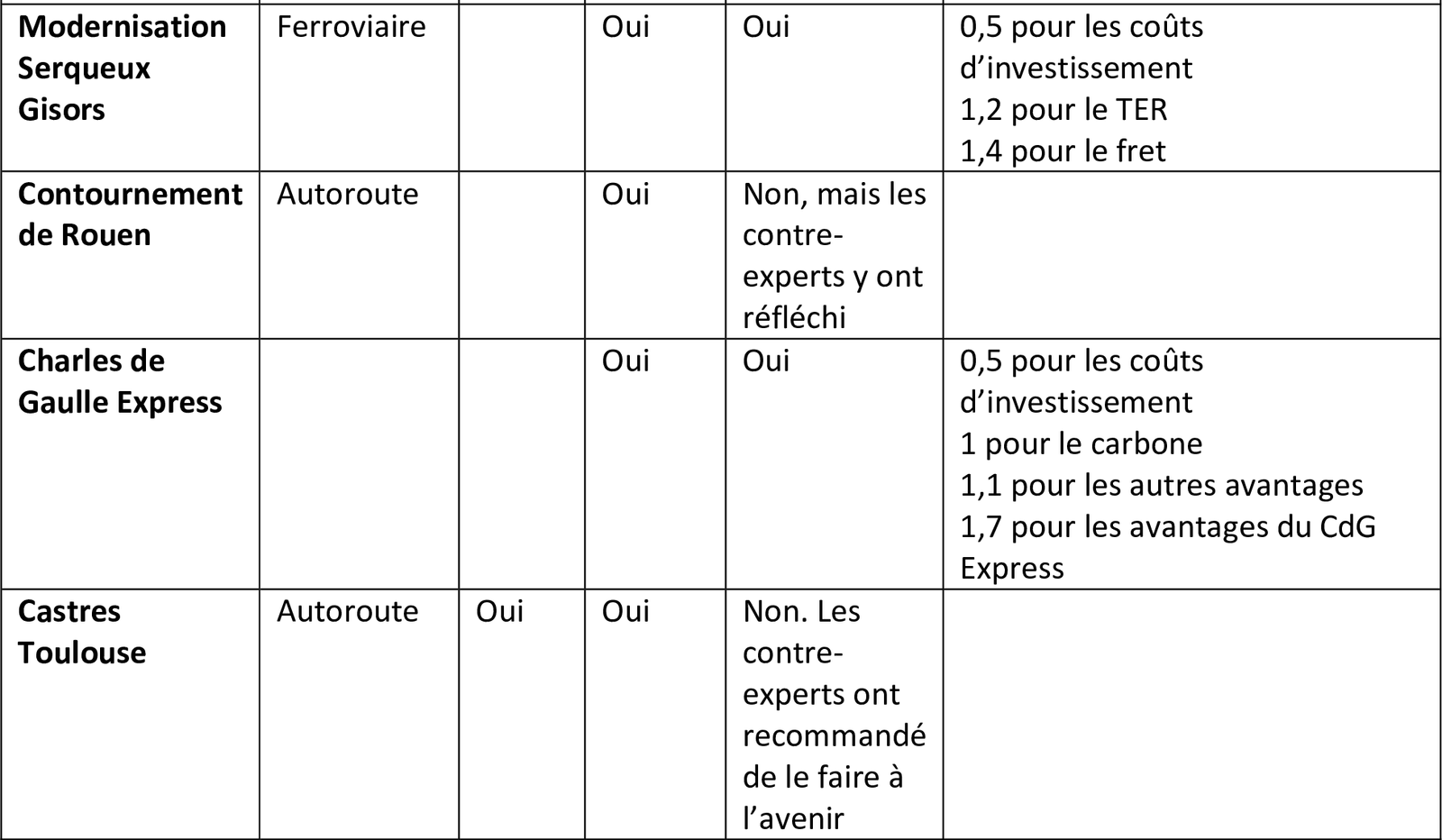
• Cadre théorique du rapport Lebègue développé dans le rapport Gollier et propose un taux d’actualisation sans risque de 2,5 % passant à 1,5 % au-delà de 2070.

• A ce taux, s’ajoute une prime de risque de 2% pondérée par un coefficient spécifique à chaque projet en fonction de la sensibilité de sa rentabilité à la croissance économique.

• Prime de risque dite systémique de 2 % est augmentée à 3 % pour les périodes d’évaluation au-delà de 2070.

Plans (1946 - 1961)

Plans (1962 - 1975)

Plans (1976 - 1985)

Plans (1986 - 1992)

Plans (1993 - 2004)

Insensibilité de l’investissement au rendement du capital

En contradiction avec néo-classique ET IS-LM

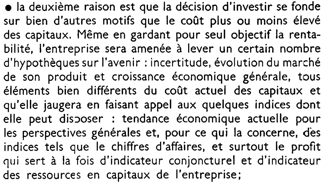
• Néo-classique: importance du coût du capital dans le modèle de Solow.

• Mais aussi: modèle IS-LM part du fait que l’investissement dépend du taux d’intérêt I(i).

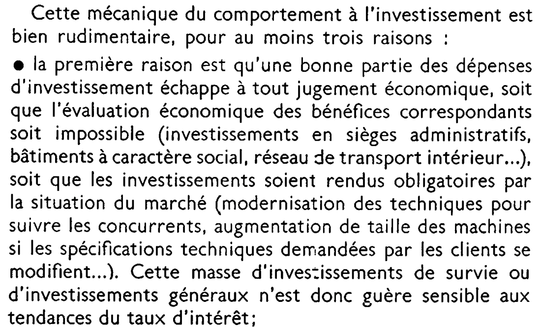
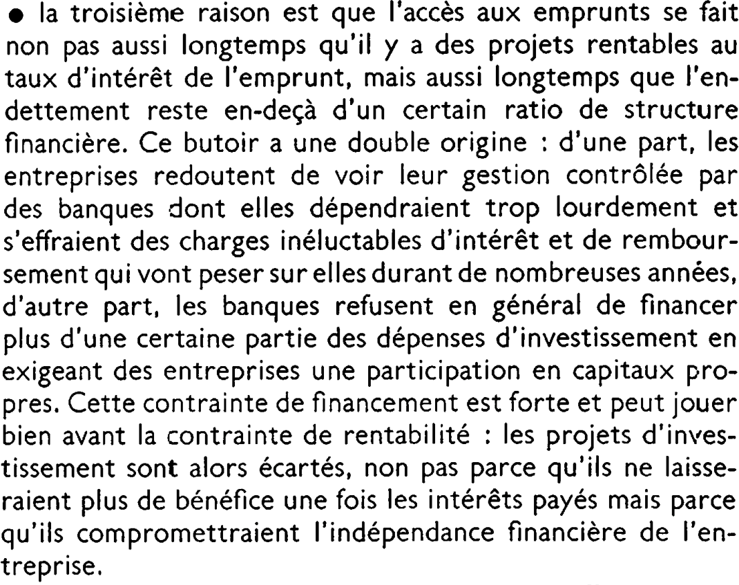
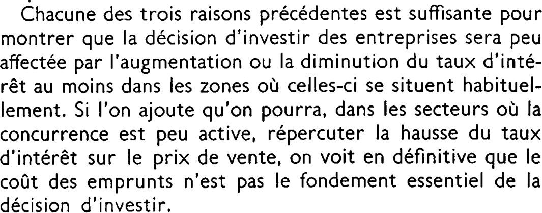
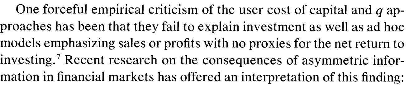
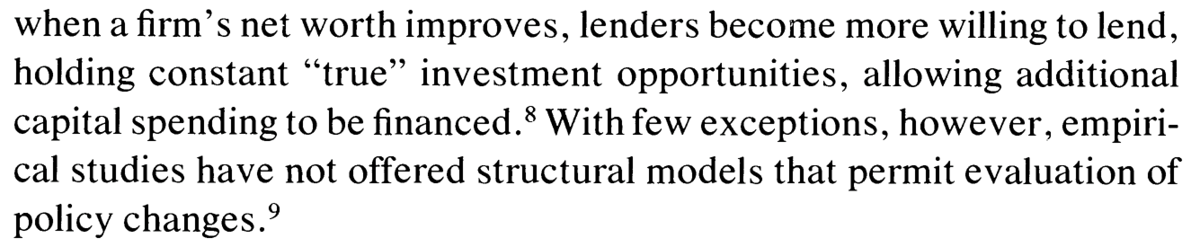
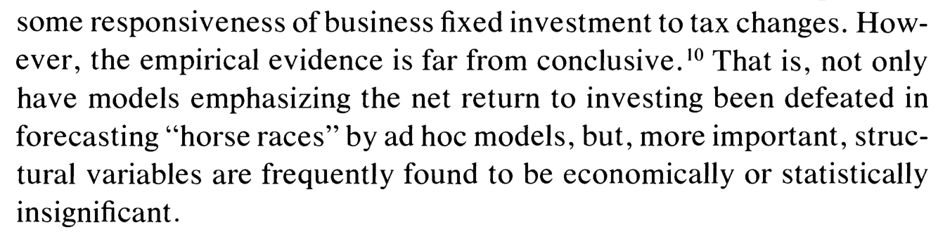
• Empiriquement: cela n’a jamais été si clair. L’effet du taux d’intérêt sur l’investissement privé est faible.

• Modèle nouveau-keynésien a remplacé cette relation par une éqauation d’Euler sur la consommation. Au contraire: la politique monétaire agit vraisemblablement via un effet redistributif passant par le marché immobilier: refinancement aux U.S., diminution des taux d’intérêt.

Stoleru (1969): dépenses qui échappent à un jugement éco

Stoleru (1969): autres motifs

Stoleru (1969): garder le contrôle

Stoleru (1969):

Actifs sûrs VS actifs risqués

Gollier (2017)

Source: Conférence France Stratégie sur le taux d’actualisation, 2017. pdf

Problématique générale

• On dit généralement que:

  • Taux actifs sûrs: 1-2%

  • Taux actifs risqués: 4-10% (selon les auteurs)

• Selon la théorie classique de la finance, cela représente une “prime de risque”. Cependant:

  • Les risques intermédiaires ne correspondent pas à des rendements intermédiaires.

  • Les risques extrêmes ne correspondent pas à des rendements supérieurs.

• Même les rendements relatifs entre classes d’actifs risqués s’expliquent mal par cette théorie:

  • Immobilier: bien moins risqué mais risque équivalent, voire supérieur.

Controverses sur l’importance de la prime de risque

• Quelle est la taille de la prime de risque?

• Handbook of Equity Risk Premium: “Returns of the Optimists”.

De la chance? Comme sur le marché immobilier parisien?

En pratique, le CAPM n’explique PAS DU TOUT les retours

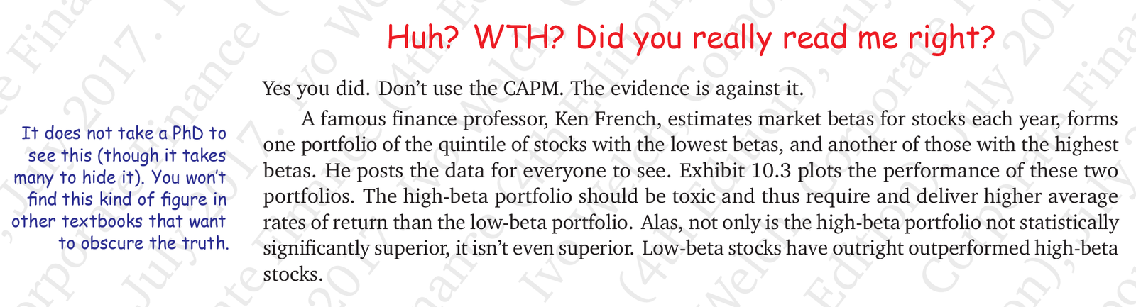
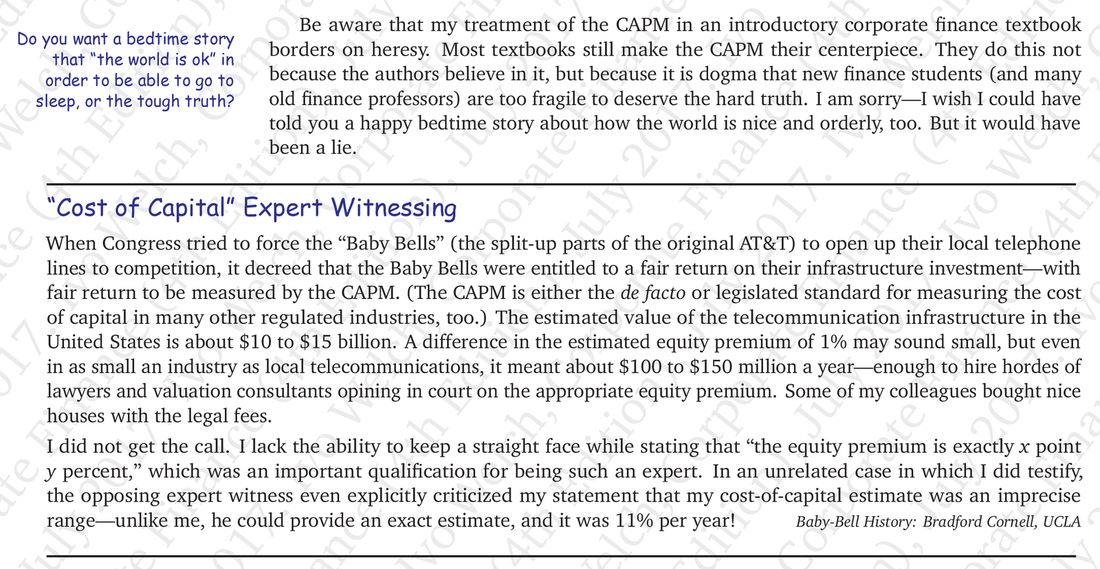
• Autre exemple: Ivo Welch, prof à UCLA.

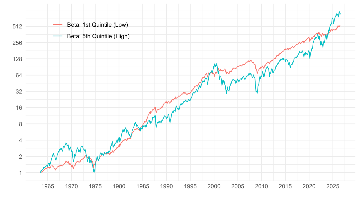
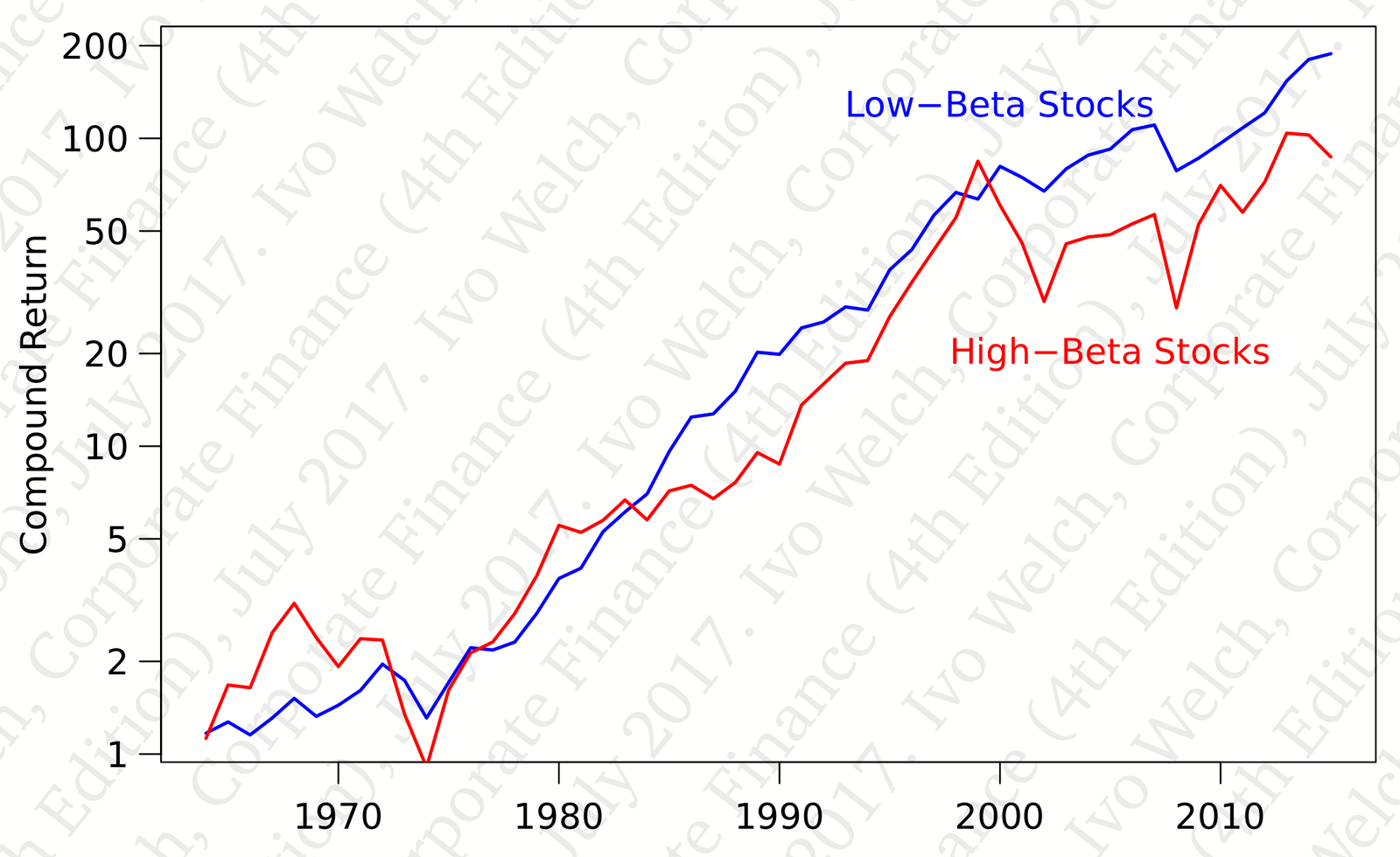
• Le CAPM marche en théorie, et il est toujours enseigné, mais c’est un échec empirique complet.

• Donc, je me demande si prendre en compte le \(\beta\) des investissements pour le public est une bonne idée.

Manuel de Ivo Welch, 2016

Manuel de Ivo Welch, 2016

Echec complet du CAPM

Ivo Welch, ancien prof à Yale, prof à UCLA

Video de Ivo Welch

Source: Livre de Corporate Finance de Ivo Welch

• Ivo Welch. pdf

Quelques exemples récents

Le cas de la Société du Grand Paris

• Source: Cour des Comptes. html

Sensibilité de la valeur des investissements au taux d’actualisation

Sensibilité de la valeur des investissements au taux d’actualisation

Dornbusch, Fischer (1979)

Successive editions

• With Startz: 2011 (11th), 2008 (10th), 2004 (9th), 2001 (8th)

• Dornbusch, Fisher

3rd edition

“the simple accelerator model does as well”

Summers et al. (1981) - Taxation and Corporate Investment: A Q-Theory Approach.

Source

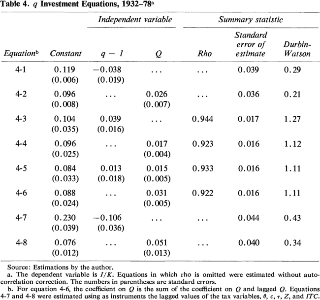
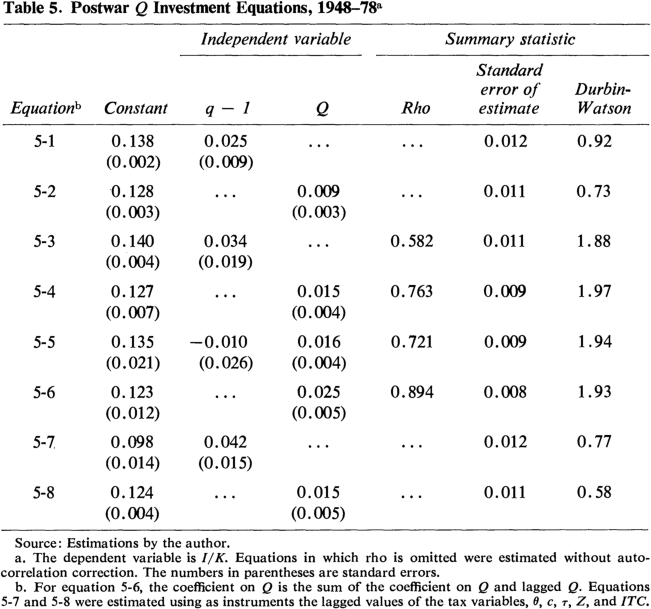
Summers, Lawrence H., Barry P. Bosworth, James Tobin, and Philip M. White. “Taxation and Corporate Investment: A Q-Theory Approach.” Brookings Papers on Economic Activity 1981, no. 1 (1981): 67–140. html / pdf

Presentation

• Summers et al. (1981) assumes a quadratic adjustment costs with constant returns. This yields the following empirical specification: \[I_{t}/K_{t}=c+b\left(q_{t}-1\right)+\epsilon_{t}.\]

• The coefficient b in this regression is the inverse of the constant term in the cost function that is: \[D\left(\frac{I}{K}\right)=\frac{1}{2b}\frac{I}{K}.\]

• The results indicate \(\hat{b}=0.031(0.005)\) which is significant, but very low: investment is not very responsive to q.

Results

Results

Shapiro (1986)

Paper

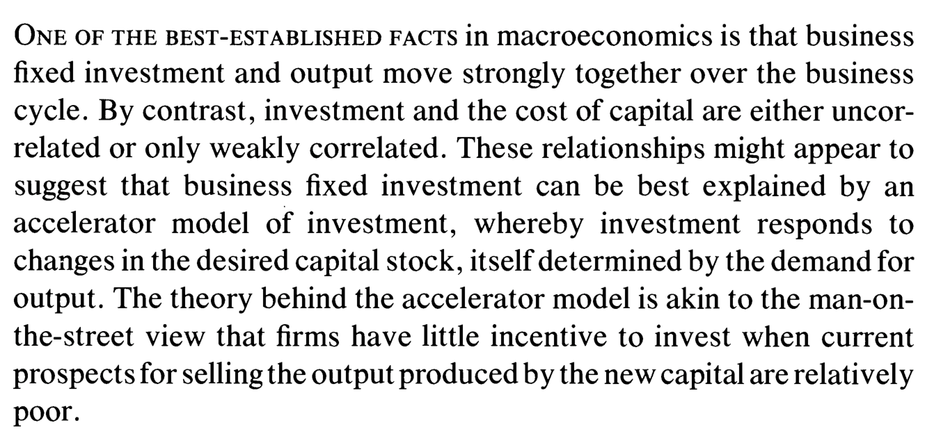
Shapiro, Matthew D., Olivier J. Blanchard, and Michael C. Lovell. “Investment, Output, and the Cost of Capital.” Brookings Papers on Economic Activity 1986, no. 1 (1986): 111–64. html / pdf

Accelerator model: “man-on-the-street view”

Inconsistent with both neoclassical and New-Keynesian

• The most important quotation in that paragraph is this:

The theory behind the accelerator model is akin to he man-on-the-street view that firms have little incentive to invest when current prospects for selling the output produced by the new capital are relatively poor.

• Shapiro (1986) rightly emphasizes:

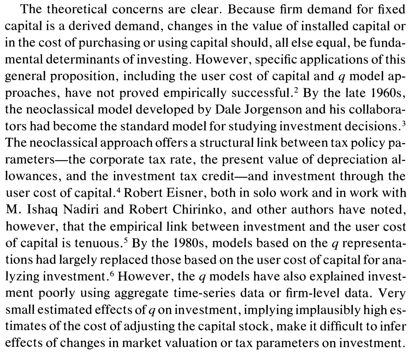
Neo-Keynesians should not, however, find comfort in this embarrassment of neoclassical theory. The textbook IS-LM model is also inconsistent with the empirical finding that output shocks rather than cost-of-capital shocks determine investment. If the interest rate does not affect investment, then the IS curve is vertical, and there is no role for the Keynesian transmission mechanism from money to output.

• I will come back to the effects of monetary policy in a future lecture.

Shapiro (1986)

Introduction

• Economists often recommend increasing investment by reducing the cost of capital through tax incentives such as accelerator depreciation and the investment tax credit.

• Anyone making such recommendations should be able to explain why output shocks seems so much important in investment dynamics than price shocks.

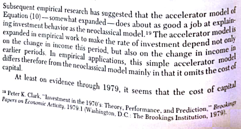
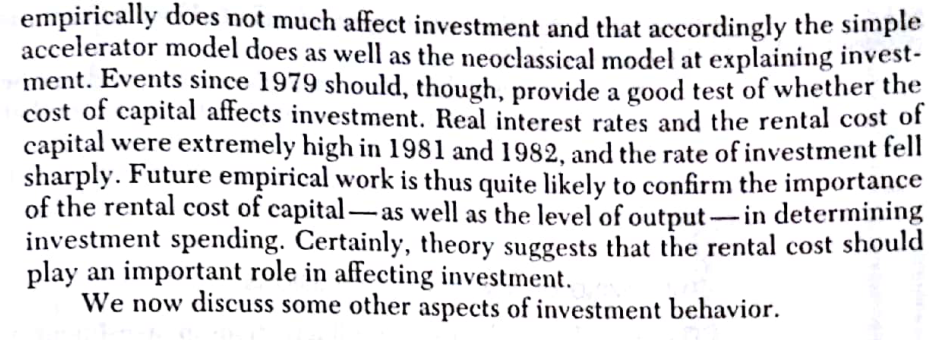
• The nation’s best-selling macroeconomics text includes the following passage:

At least on evidence through 1979; it seems that the cost of capital empirically does not much affect investment and that accordingly the simple accelerator model does as well as the neoclassical model at explaining investment.

Blanchard’s discussion

• “The discrepancy between theory and empirical work is perhaps nowhere in macroeconomics so obvious as in the case of the aggregate investment function.”

• The theory from which the neoclassical investment function was initially derived implies that one should be able to specify the model equally well whether using only factor prices or using output and the user cost of capital. We all know that this is not the case.

• It is very hard to make sense of the distributed lag of output on investment.

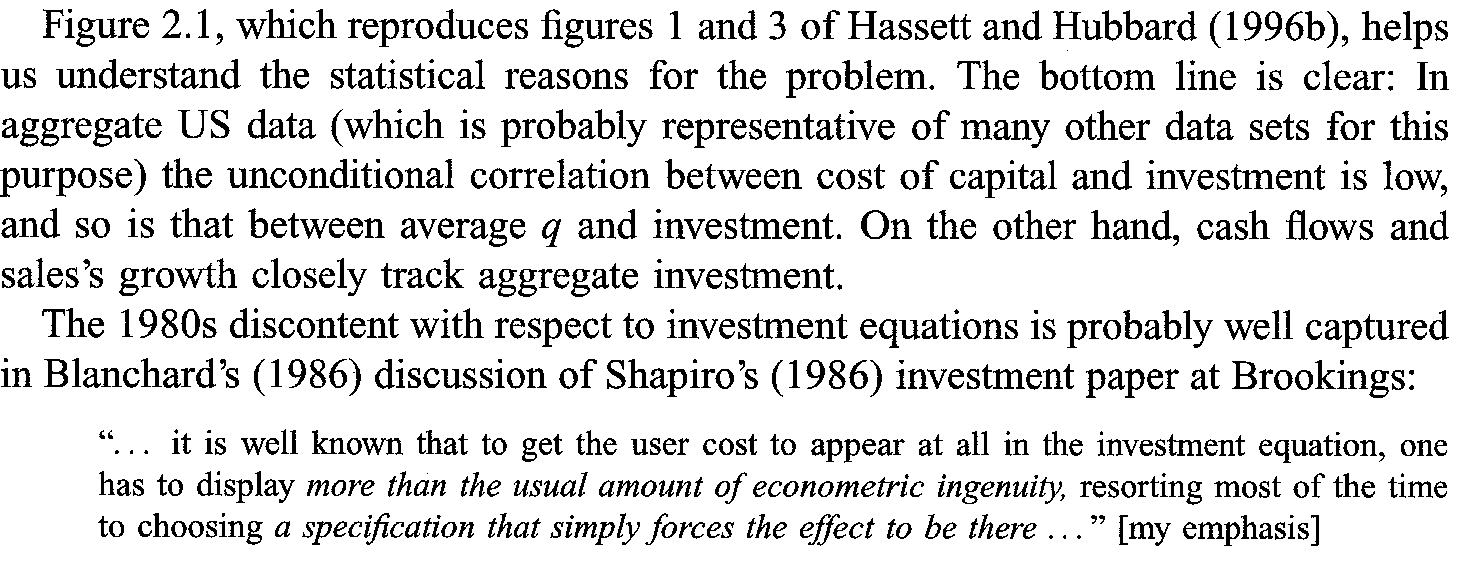
• Finally, it is well known that to get the user cost to appear at all in the investment equation, one has to display more than the usual amount of econometric ingenuity, resorting most of the time to choosing a specification that simply forces the effect to be there.

Cummins, Hassett, Hubbard (1994)

Paper

Cummins, Jason G., Kevin A. Hassett, R. Glenn Hubbard, Robert E. Hall, and Ricardo J. Caballero. “A Reconsideration of Investment Behavior Using Tax Reforms as Natural Experiments.” Brookings Papers on Economic Activity 1994, no. 2 (1994): 1–74. html / pdf

Introduction

Literature

Literature

Hall’s discussion

• Instrument \(q\) using changes in the tax code. The idea is that changes in taxes can have large effects on a firms valuation and will differ across industries depending on capital intensity. So using changes in the tax code, they estimate a \(\hat{b}\) close to 0.5 on firm level data (Compustat), which implies that the adjustment costs are more reasonable, around 4 % of capital. However, it is unclear how much this result carries over to aggregate investment:

1. To the extent that the supply of investment goods is not infinitely elastic, the effect of an increased demand for capital may be mostly to raise the price of investment goods.

2. the \(R^{2}\) of the regressions are quite low, i.e. q still explains a small fraction of investment at the firm level. In fact, the \(R^{2}\) increase significantly once we add cash flow or other current variables (current profits, current sales) as a right hand side variable, the fit improves markedly.

Caballero’s discussion

Like so many other papers in the investment literature, this one starts by summarizing the empirical failure of models that emphasize the role of “price” variables in investment equations and by listing the standard culprits (simultaneity, error in variables, and so forth). Unlike many others, it concludes on a very positive note. By isolating the “exogenous” cross-sectional elements of episodes covering important tax reforms, the authors claim to have eluded the standard problems and found evidence of a large short-run response of investment to price incentives.

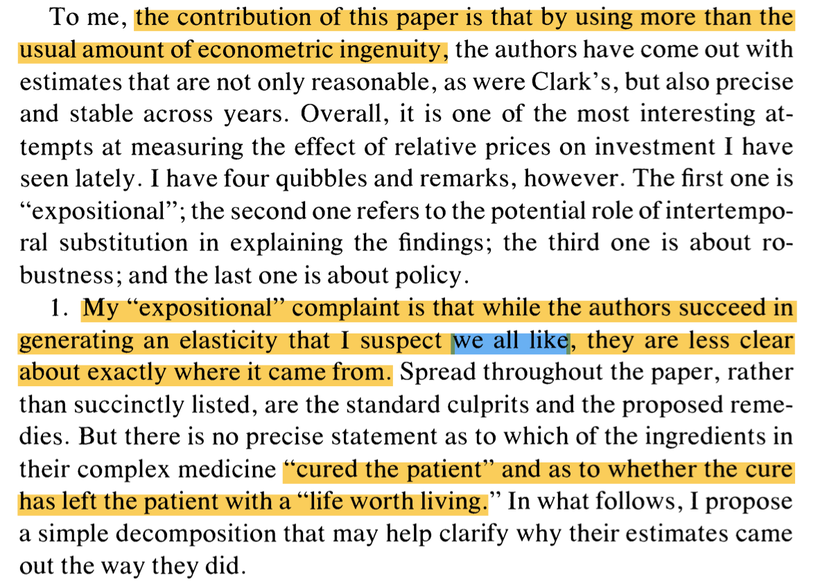
My “expositional” complaint is that while the authors succeed in generating an elasticity that I suspect we all like, they are less clear about exactly where it came from.

“An elasticity that I suspect we all like”

Poterba, Summers (1995)

Paper

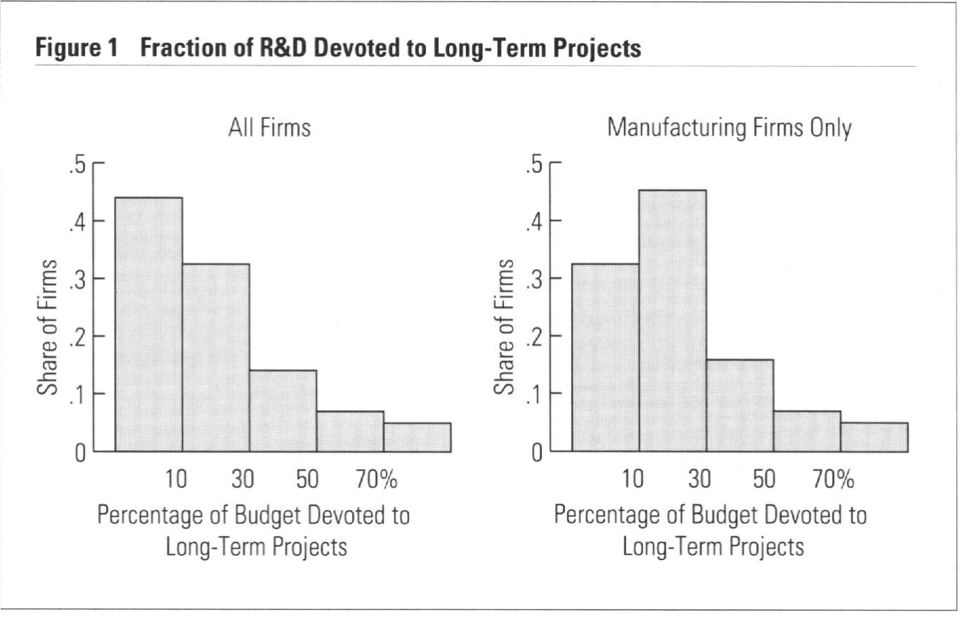
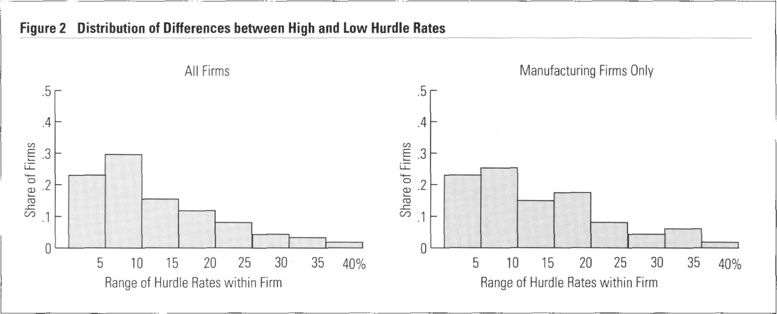
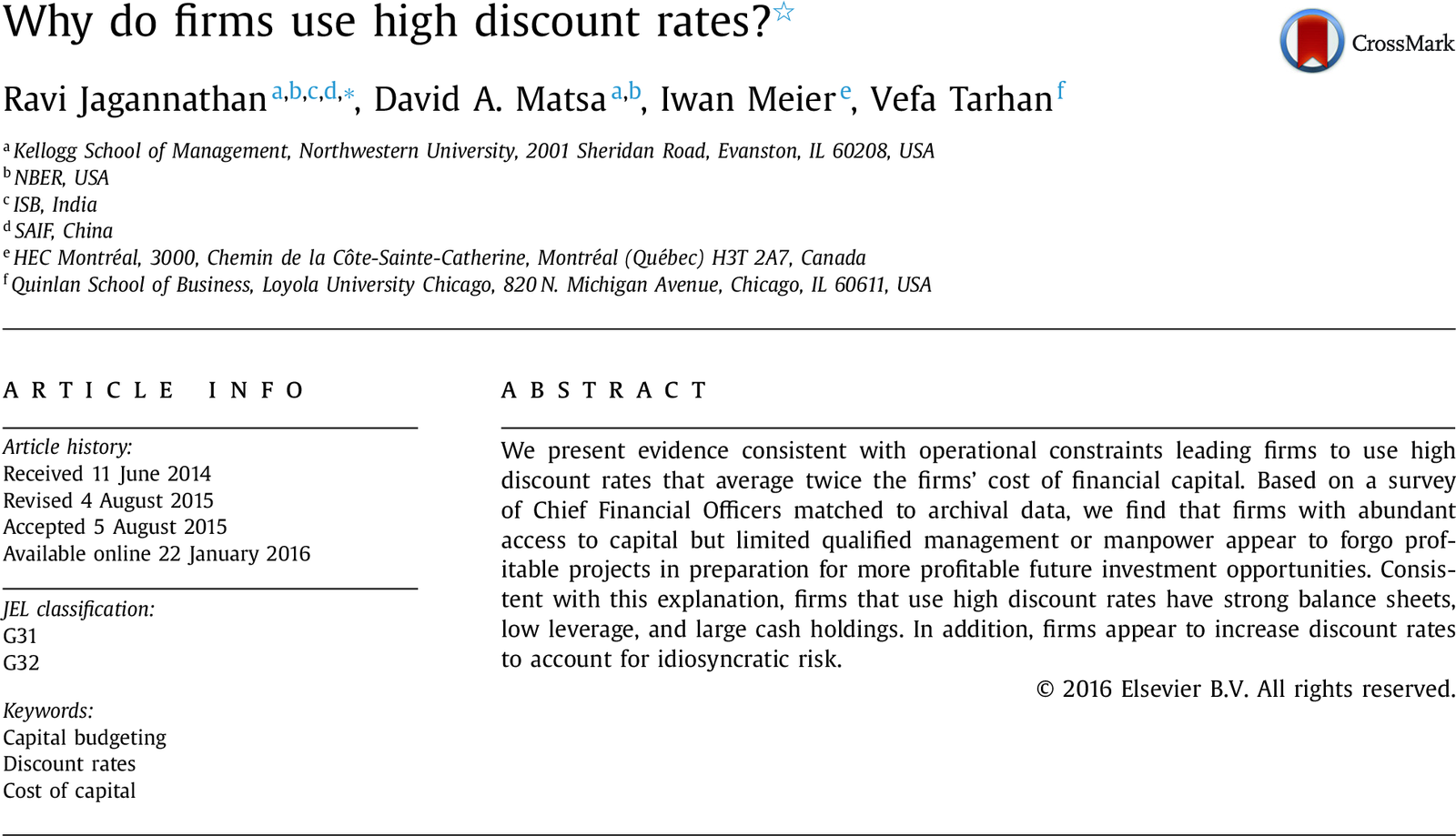
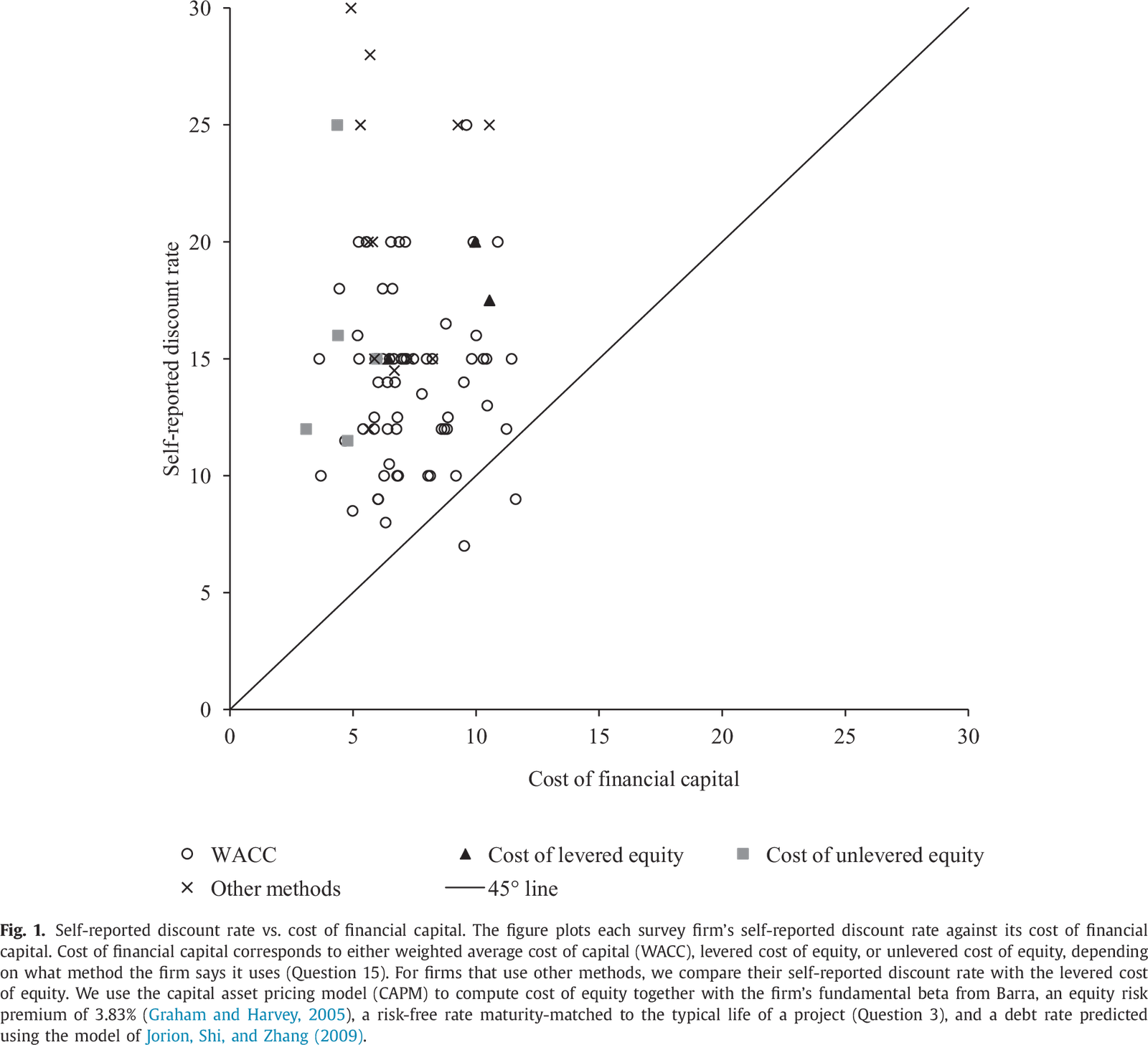
Poterba, J. M., & Summers, L. H. (1995). A Ceo Survey of U.s. Companies’ Time Horizons and Hurdle Rates. Sloan Management Review, 37(1), 43–53. pdf / html

Themes

• Hurdle rates used in capital budgeting decisions.

• Higher hurdle rates to correct for over-optimistic assessments of Free Cash Flows: this leads to short-termism on the part of U.S. Manufacturing Firms.

• Different hurdle rates within a firm, unrrelated to risk: entering new markets, defending market shares have lower hurdle rates.

• Hurdle rates not related to cross-sectional risk.

Very interesting paper

Very interesting paper

Figure 2

Caballero (1999) - Aggregate Investment

Paper

Caballero, Ricardo J. “Chapter 12 Aggregate Investment.” In Handbook of Macroeconomics, 1:813–62. Elsevier, 1999. html / pdf

Quotes on theory against empirics

• What if the right model is one where the capital stock is not interest elastic?

Neoclassical model rejected in 1980s

q-model lack empirical success

• “Scale variables” such as cash-folows always seemed to matter more in investment equations than \(q\) which should have been a sufficient statistic.

Econometric “ingenuity”?

Low frequency is the only data point

• Usual argument in favor of neoclassical model: Kaldor facts.

Yagan (2015) - 2003 Dividend Tax Cut

Abstract

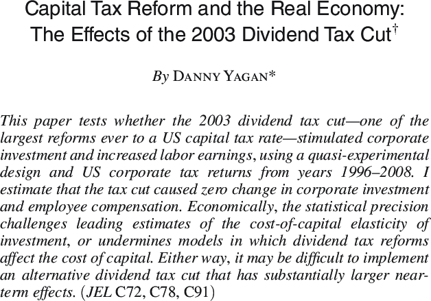
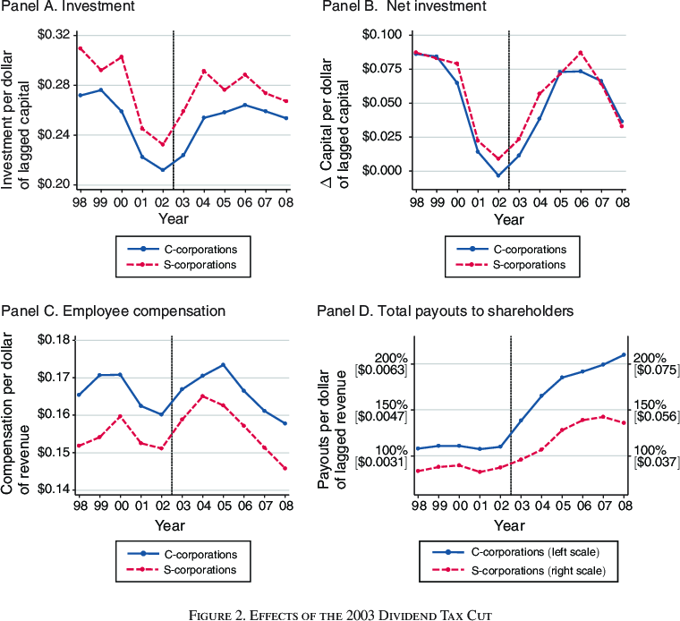
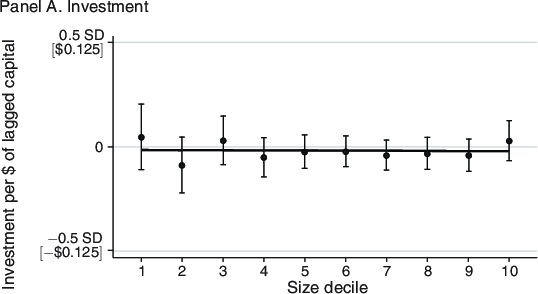
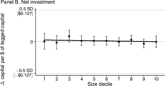
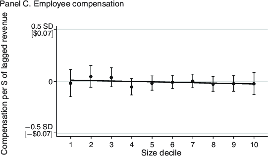
This paper tests whether the 2003 dividend tax cut—one of the largest reforms ever to a US capital tax rate—stimulated corporate investment and increased labor earnings, using a quasi-experimental design and US corporate tax returns from years 1996–2008. I estimate that the tax cut caused zero change in corporate investment and employee compensation. Economically, the statistical precision challenges leading estimates of the cost-of-capital elasticity of investment, or undermines models in which dividend tax reforms affect the cost of capital. Either way, it may be difficult to implement an alternative dividend tax cut that has substantially larger near-term effects.

Abstract

Presentation

• The Jobs and Growth Tax Relief Reconciliation Act of 2003 reduced the top federal tax rate on individual dividend income in the United States from 38.6 % to 15 %.

• Difference in difference: \[INV_{it}=\alpha_{1}CCORP_{i,t-2}+\alpha_{2}CCORP_{i,t-2}\times POST_{t}+\mathbf{X}_{i,t-2}\beta+\mathbf{YEAR_{t}}\gamma.\]

• Real corporate outcomes are too cyclical to distinguish tax effects from business cycle effects.

Presentation

• Aggregate investment rose 31 % in the five years after the tax cut, but that increase could have been driven by secular emergence from the early 2000s recession.

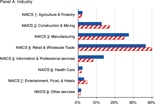
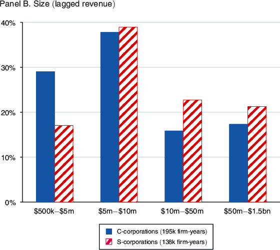
• C-corporations and S-corporations face similar tax rates except that C-corporations are subject to dividend taxation while S-corporations are not.

• This paper uses S-corporations (not directly affected by the dividend tax cut) as a control group for C-corporations (directly affected) over time.

Compare sectors

Compare sizes

Compare investment: C vs. S corporations

Compare Investment

Compare Net Investment

Compare Compensation

Jagannathan, Matsan, Meier, Tarhan (2016)

Figure 4

Figure 4

JP Morgan (2016)

Paper

Figure 4

Figure 5

Sharpe, Suarez (2020)

Paper

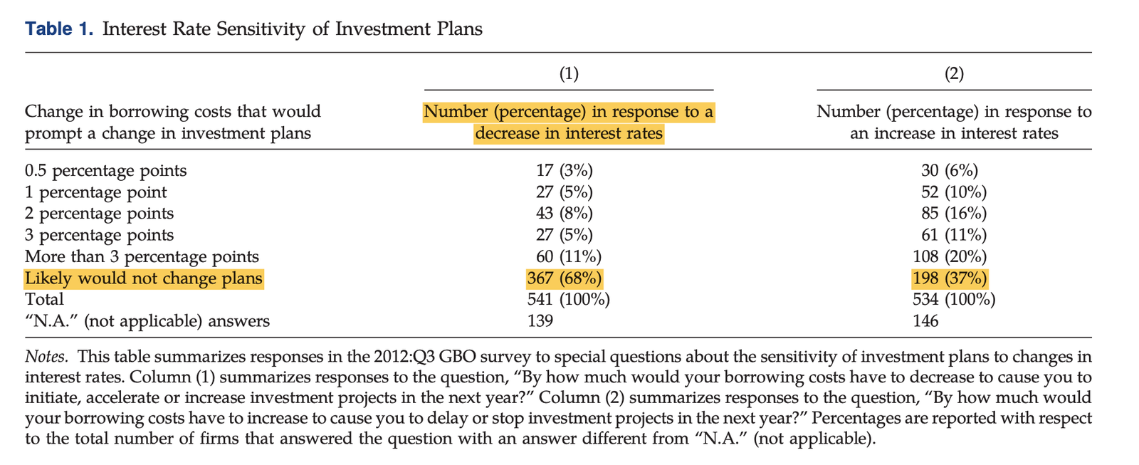
Sharpe, S. A., & Suarez, G. A. (2021). Why Isn’t Business Investment More Sensitive to Interest Rates? Evidence from Surveys. Management Science, 67(2), 720–741. pdf / html

Figure 1

Interest Rate Sensitivity of Investment Plans

Reasons for Insensitivity to Interest Rate Changes

Back to secular stagnation ?

Paper

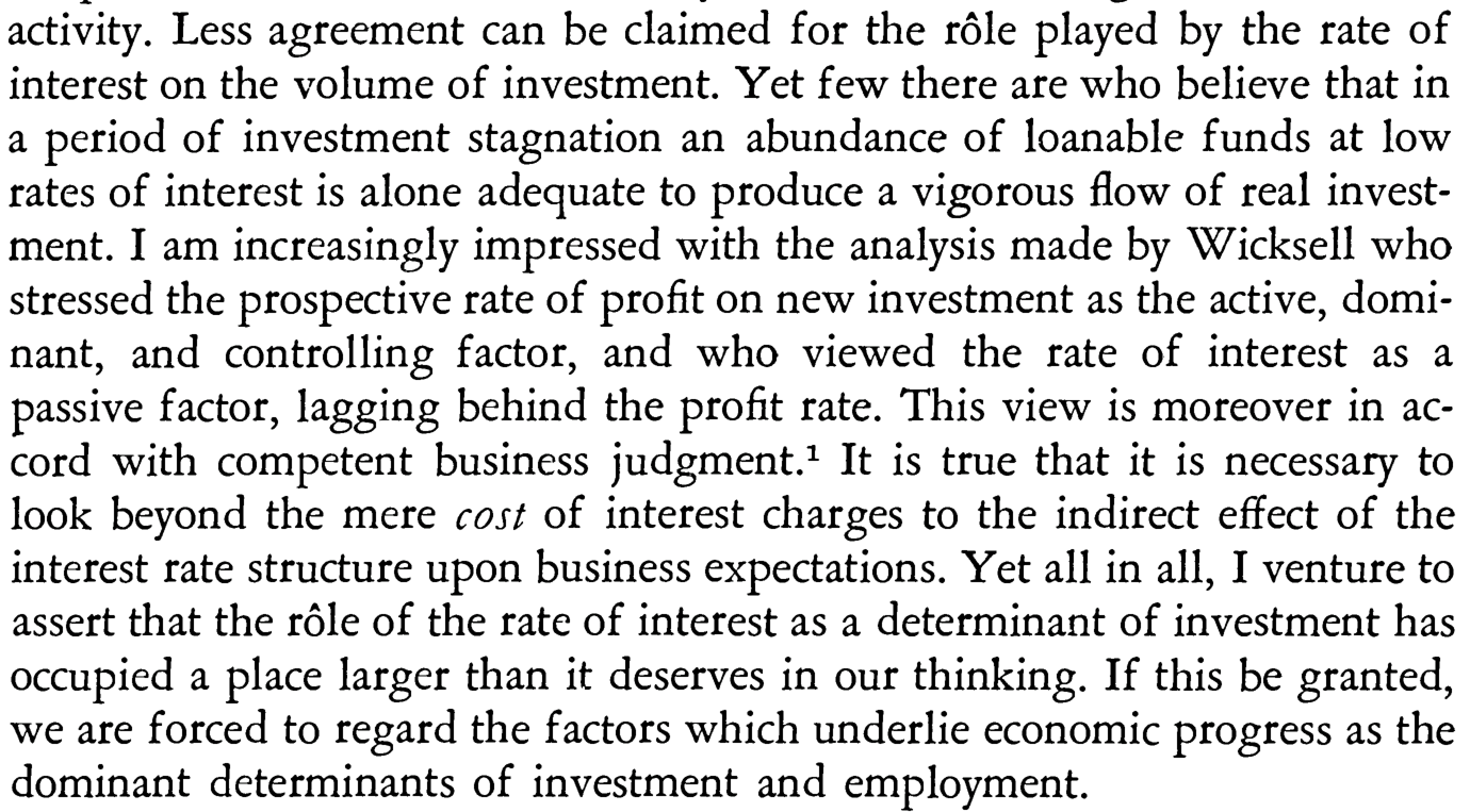
Hansen, Alvin H. “Economic Progress and Declining Population Growth.” The American Economic Review 29, no. 1 (1939): 1–15. html / pdf

Investment is not that interest elastic

Other quotes from the address

• The role of the rate of interest in the determination of investment has perhaps been overstated.

• Hansen favored the investigation of new investment outlets:

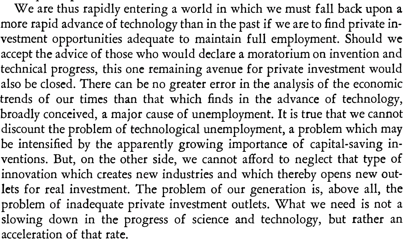
The problem of our generation is, above all, the problem of inadequate private investment outlets. What we need is not a slowing down in the progress of science and technology, but rather an acceleration of that rate.

Technological unemployment

Deepening VS Widening of capital

According to Douglas, the growth of real capital formation in England from 1875 to 1909 proceeded at an average rate of two per cent per annum; and the rate of growth of capital formation in the United States from 1890 to 1922 was four per cent per annum. The former is less than the probable rate of increase of output in England, while the latter is somewhat in excess of the annual rise of production in the United States. Thus, during the last fifty years or more, capital formation for each economy as a whole has apparently consisted mainly of a widening of capital. Surprising as it may seem, as far as we may judge from such data as are available, there has been little, if any, deepening of capital. The capital stock has increased approximately in proportion to real income.

Conclusions: what do we know ?

Consumption: main takeways

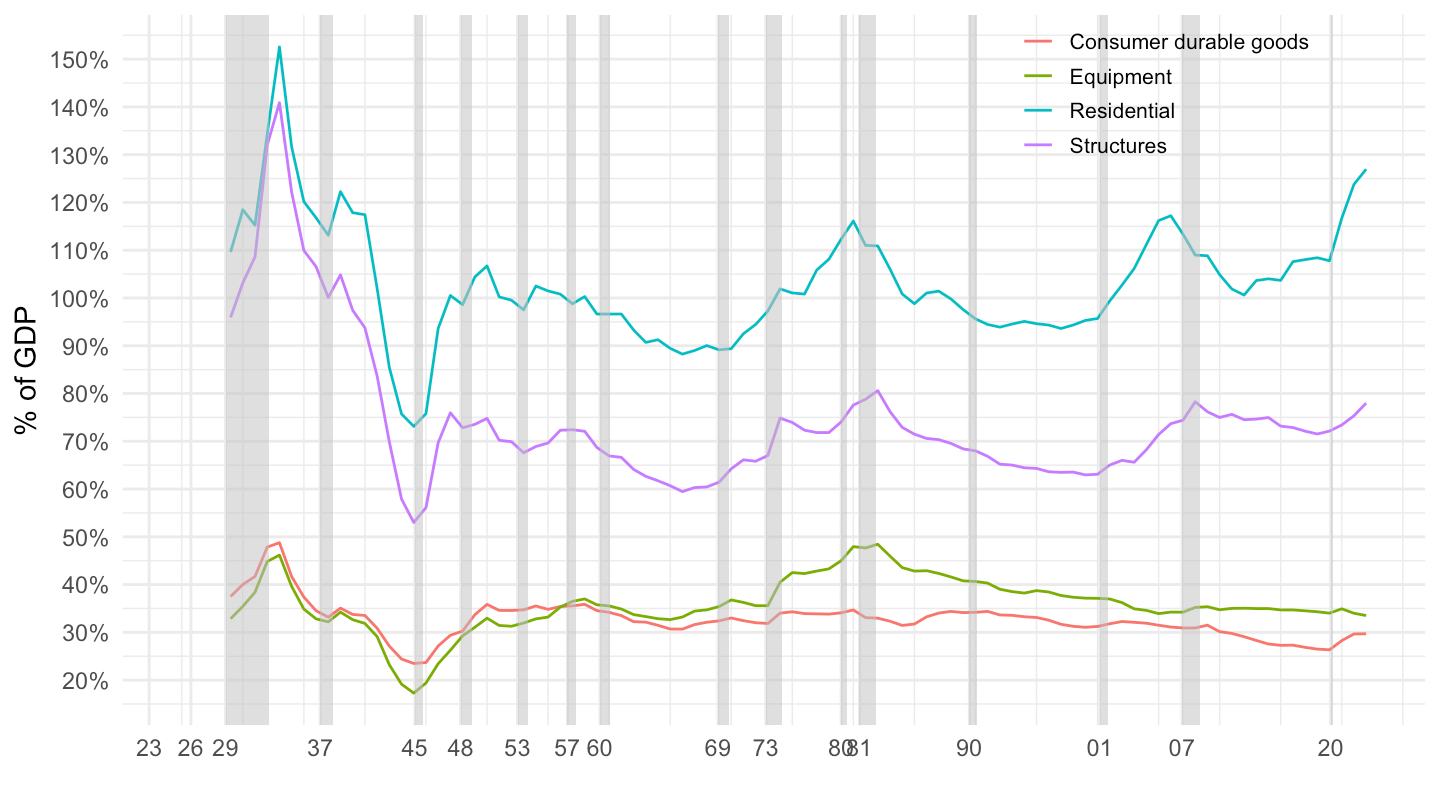
• Importance of saving rates / MPCs by income groups. (which are persistent) “Ad-hoc” consumption functions ?

• Consumption responds to income even when shocks to income was anticipated. (expectations probably have too much weight in the discussion)

• Housing wealth effects ?

• Failure of the Euler equation does not arise solely from incomplete markets.

• People expose themselves to risk. (adjustable rate mortgages)

• Evidence for housing wealth effects is not totally convincing.

Investment: main takeaways

• Interest rates / “Cost of capital” has small effects. Scale variables count much more. “Accelerator” (demand) or “financial accelerator” (constraints) ?

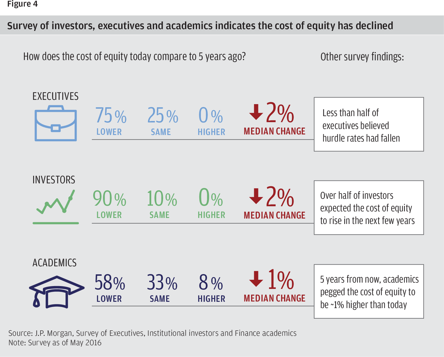
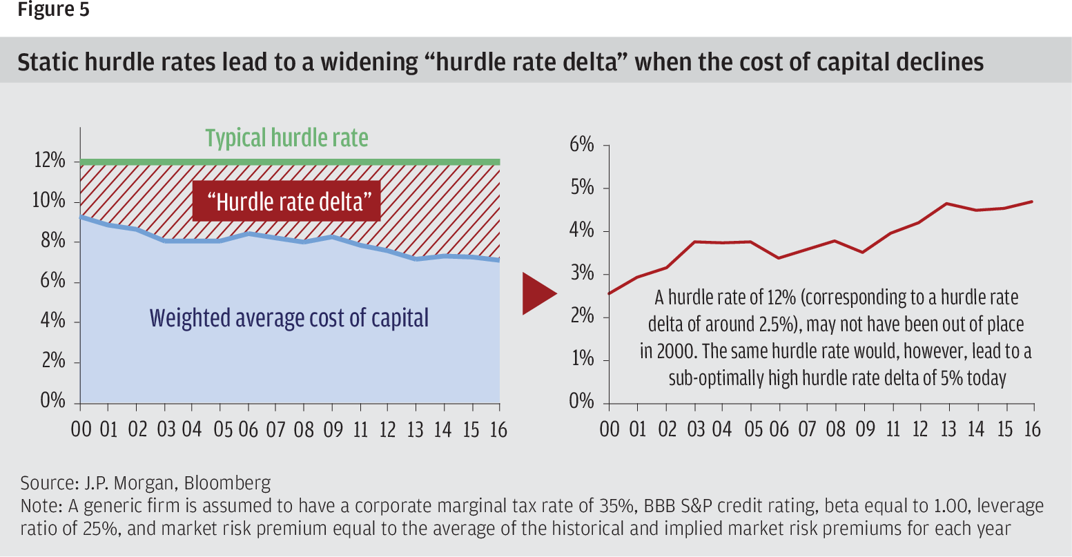
• Hurdle rates move little with interest rates.

• Asks questions about asset pricing?

• Open economy: gets even worse. Capital goes the wrong way.

• Asset pricing: solutions to “puzzles” for asset pricing create new ones for investment. Problem of production-based asset pricing.

• The really interesting data analysis is probably at the intersection between macro and finance, macro and international, macro / finance / international.

Bibliography

Bibliography