CAC 40
Data - Yahoo
Info
LAST_COMPILE
| LAST_COMPILE |
|---|
| 2026-07-24 |
Last
| date | Nobs |
|---|---|
| 2026-07-23 | 39 |
symbol
Dividendes
BNP Paribas
Code
CAC40_dividendes %>%
  filter(`Intitulé` %in% c("BNP Paribas")) %>%
  select(2, 7, 8, 9, 10) %>%
  print_table_conditional()
Vinci
Code
CAC40_dividendes %>%
  filter(`Intitulé` %in% c("Vinci")) %>%
  select(2, 7, 8, 9, 10, 11, 12) %>%
  print_table_conditional()
Components
1990-
Linear
Code
plot_linear <- CAC40 %>%
  left_join(CAC40_components, by = "symbol") %>%
  filter(symbol %in% c("DSY", "HO")) %>%
  filter(date >= as.Date("1990-01-01")) %>%
  group_by(symbol) %>%
  arrange(date) %>%
  mutate(close = 100*close/close[1]) %>%
  ggplot() + geom_line(aes(x = date, y = close, color = Symbol)) +
  theme_minimal() + xlab("") + ylab("") +
  theme(legend.title = element_blank(),
        legend.position = c(0.5, 0.9)) +
  scale_y_continuous(breaks = seq(0, 1000000, 100)) +
  scale_x_date(breaks = as.Date(paste0(seq(1945, 2100, 5), "-01-01")),
               labels = date_format("%Y"))

plot_linear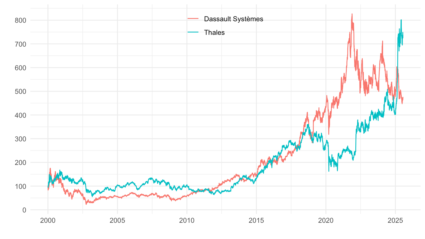
Log
Code
plot_log <- plot_linear +
  scale_y_log10(breaks = c(50, 80, 100,200, 500, 800, 1000))

plot_log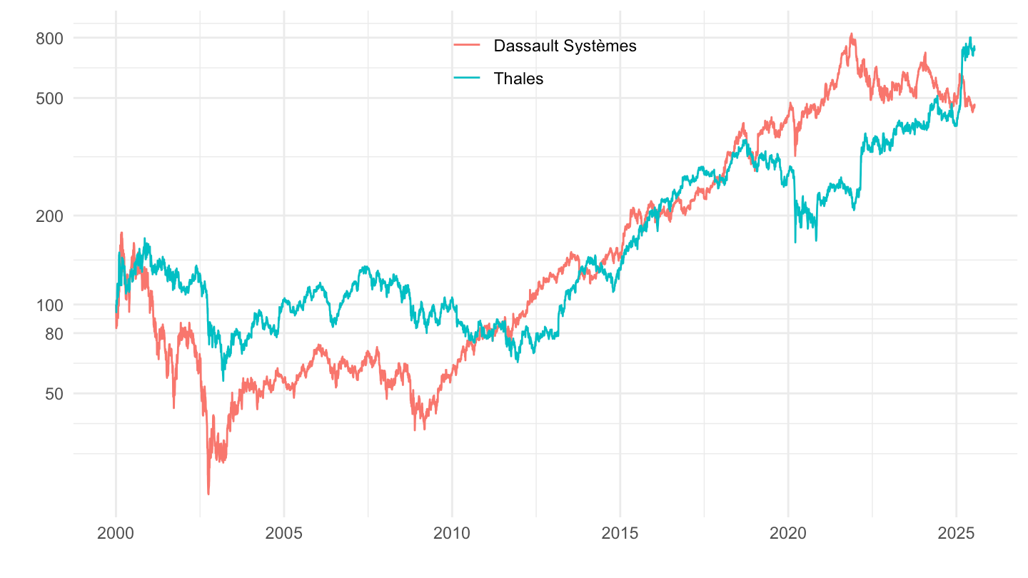
Bind
Code
ggpubr::ggarrange(plot_linear + ggtitle("Linear scale"), plot_log + ggtitle("Log scale"), common.legend = T)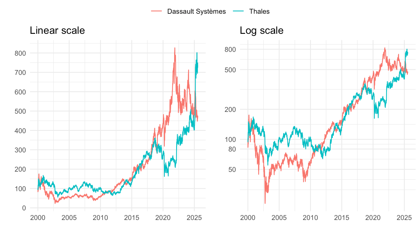
2010-
Linear
Code
plot_linear <- CAC40 %>%
  left_join(CAC40_components, by = "symbol") %>%
  filter(symbol %in% c("LR", "MC")) %>%
  filter(date >= as.Date("2010-01-01")) %>%
  group_by(symbol) %>%
  arrange(date) %>%
  mutate(close = 100*close/close[1]) %>%
  ggplot() + geom_line(aes(x = date, y = close, color = Symbol)) +
  theme_minimal() + xlab("") + ylab("") +
  theme(legend.title = element_blank(),
        legend.position = c(0.2, 0.7),
        axis.text.x = element_text(angle = 45, vjust = 0.5, hjust=1)) +
  scale_y_continuous(breaks = seq(0, 1000000, 100),
                     labels = dollar_format(pre = "", acc = 1)) +
  scale_x_date(breaks = as.Date(paste0(seq(1940, 2100, 1), "-01-01")),
               labels = date_format("%Y"))

plot_linear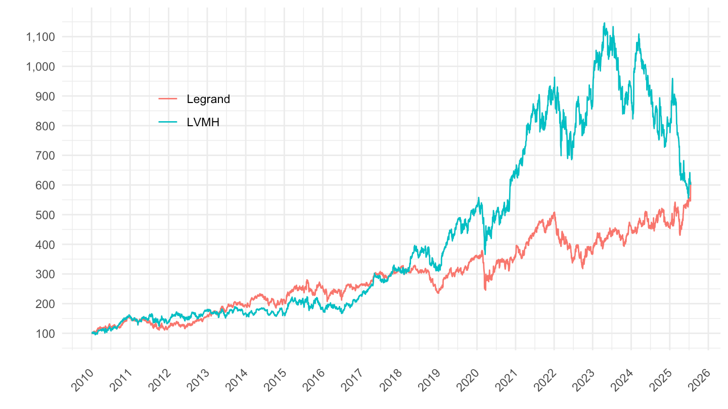
Log
Code
plot_log <- plot_linear +
  scale_y_log10(breaks = c(10^seq(1, 100, 1), 10^seq(1, 100, 1)*2, 10^seq(1, 100, 1)*5),
                     labels = dollar_format(pre = "", acc = 1))

plot_log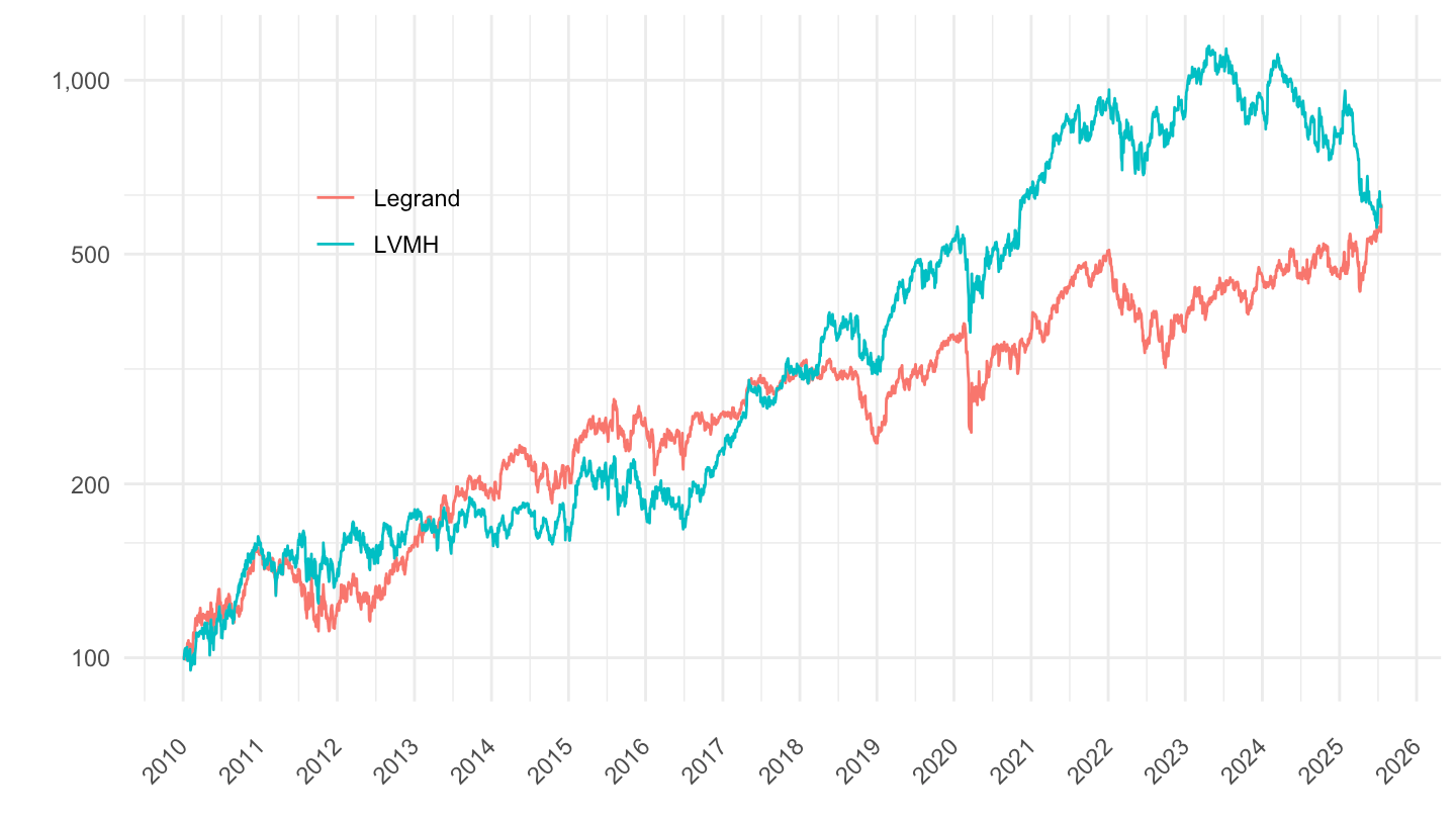
Bind
Code
ggpubr::ggarrange(plot_linear + ggtitle("Linear scale"),
                  plot_log + ggtitle("Log scale"),
                  common.legend = T)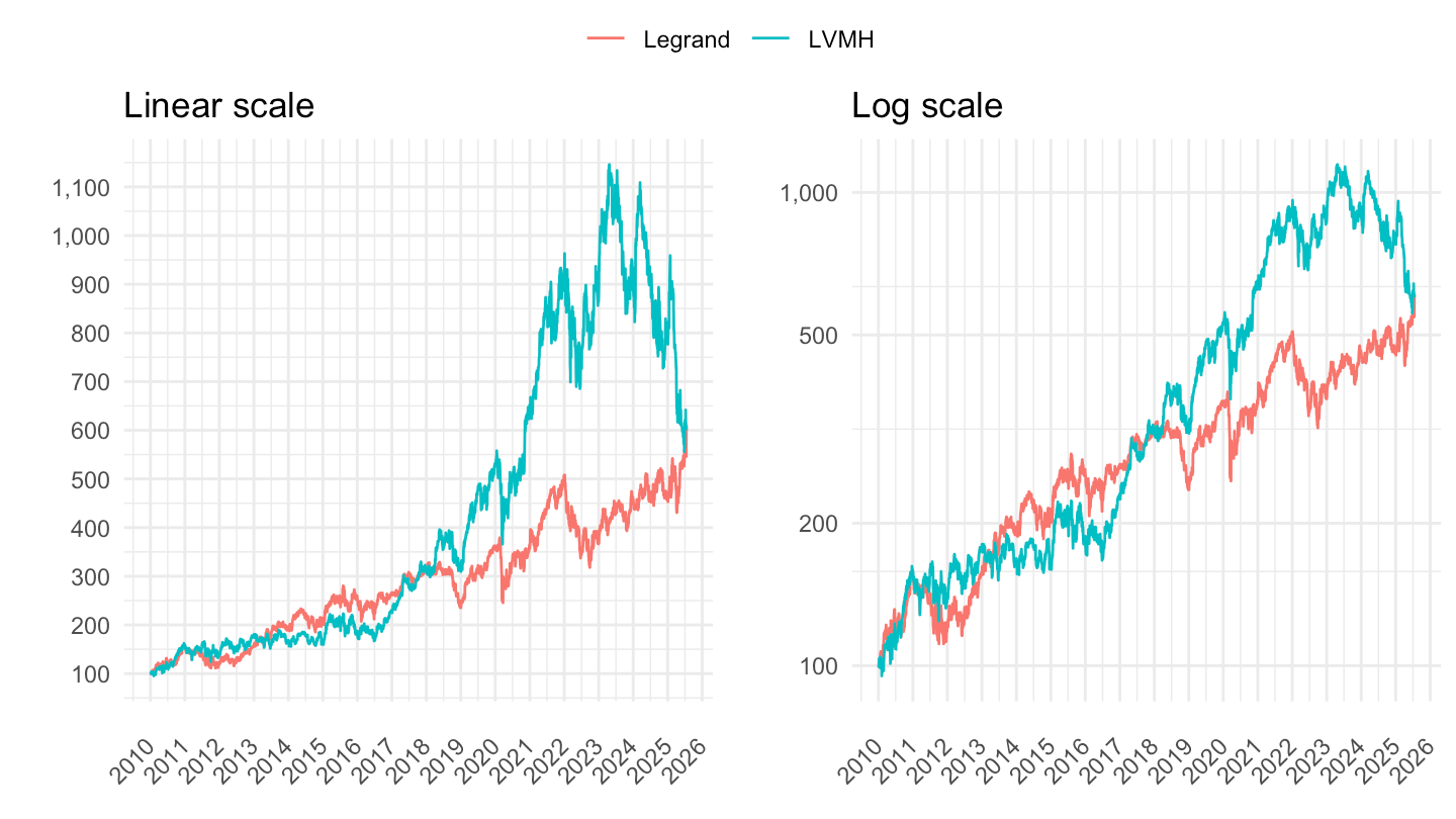
2014-
Linear
Code
plot_linear <- CAC40 %>%
  left_join(CAC40_components, by = "symbol") %>%
  filter(symbol %in% c("DSY", "HO")) %>%
  filter(date >= as.Date("2014-01-01")) %>%
  group_by(symbol) %>%
  arrange(date) %>%
  mutate(close = 100*close/close[1]) %>%
  ggplot() + geom_line(aes(x = date, y = close, color = Symbol)) +
  theme_minimal() + xlab("") + ylab("") +
  theme(legend.title = element_blank(),
        legend.position = c(0.2, 0.7),
        axis.text.x = element_text(angle = 45, vjust = 0.5, hjust=1)) +
  scale_y_continuous(breaks = seq(0, 1000000, 100),
                     labels = dollar_format(pre = "", acc = 1)) +
  scale_x_date(breaks = as.Date(paste0(seq(1940, 2100, 1), "-01-01")),
               labels = date_format("%Y"))

plot_linear
Log
Code
plot_log <- plot_linear +
  scale_y_log10(breaks = c(10^seq(1, 100, 1), 10^seq(1, 100, 1)*2, 10^seq(1, 100, 1)*5),
                     labels = dollar_format(pre = "", acc = 1))

plot_log
Bind
Code
ggpubr::ggarrange(plot_linear + ggtitle("Linear scale"),
                  plot_log + ggtitle("Log scale"),
                  common.legend = T)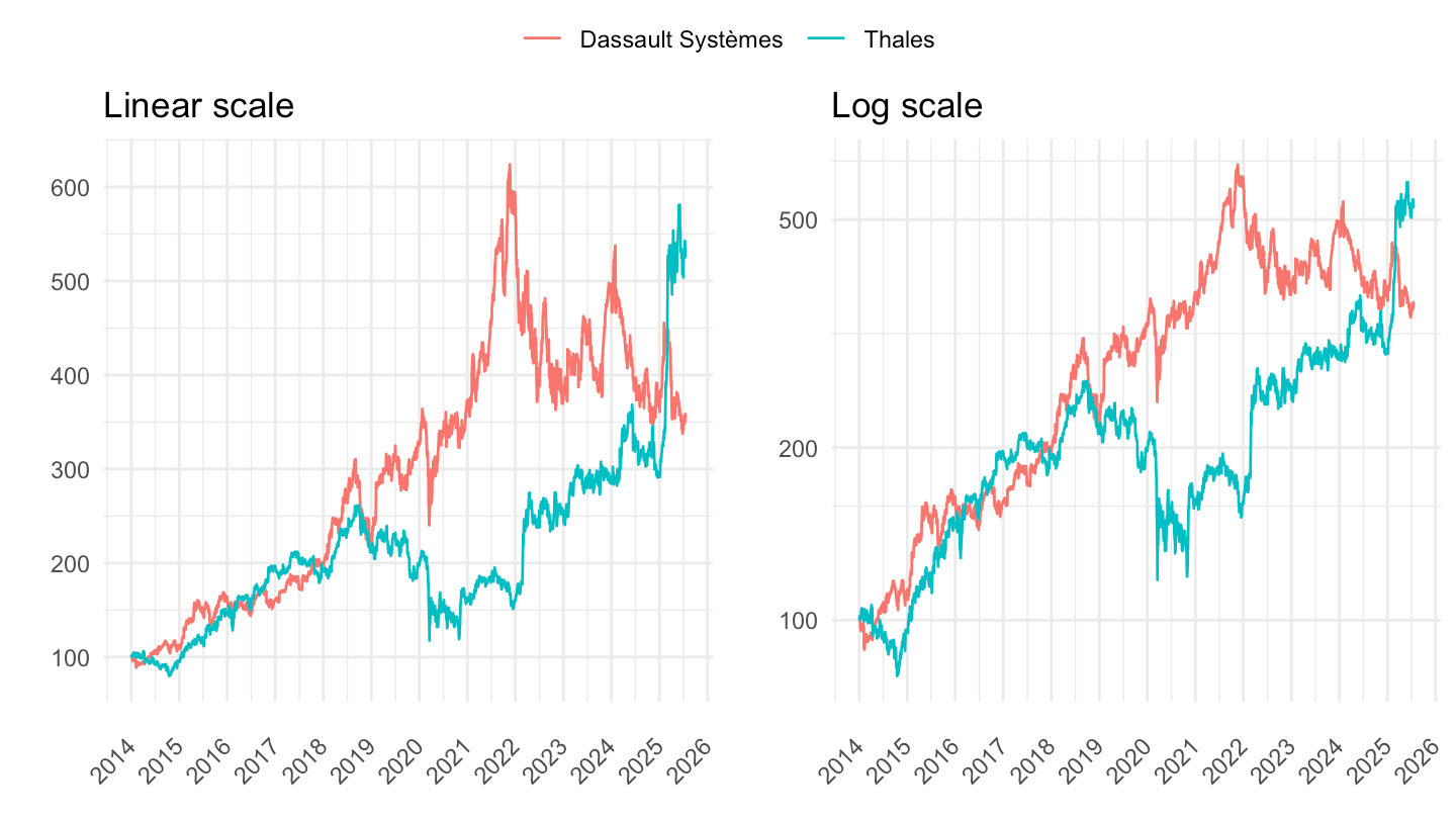
Banques
Tous
Code
CAC40 %>%
  left_join(CAC40_components, by = "symbol") %>%
  filter(symbol %in% c("BNP", "ACA", "GLE")) %>%
  #filter(date >= as.Date("1990-01-01")) %>%
  ggplot + geom_line(aes(x = date, y = close, color = Symbol)) +
  theme_minimal() + xlab("") + ylab("Stock Price (Close)") +
  scale_x_date(breaks = seq(1960, 2100, 2) %>% paste0("-01-01") %>% as.Date,
               labels = date_format("%Y")) +
  scale_y_log10(breaks = c(1, 2, 3, 5, 10, 25, 50, 100, 200, 500),
                     labels = dollar_format(prefix = "", suffix = "€", accuracy = 1)) +
  theme(legend.position = c(0.2, 0.80),
        legend.title = element_blank())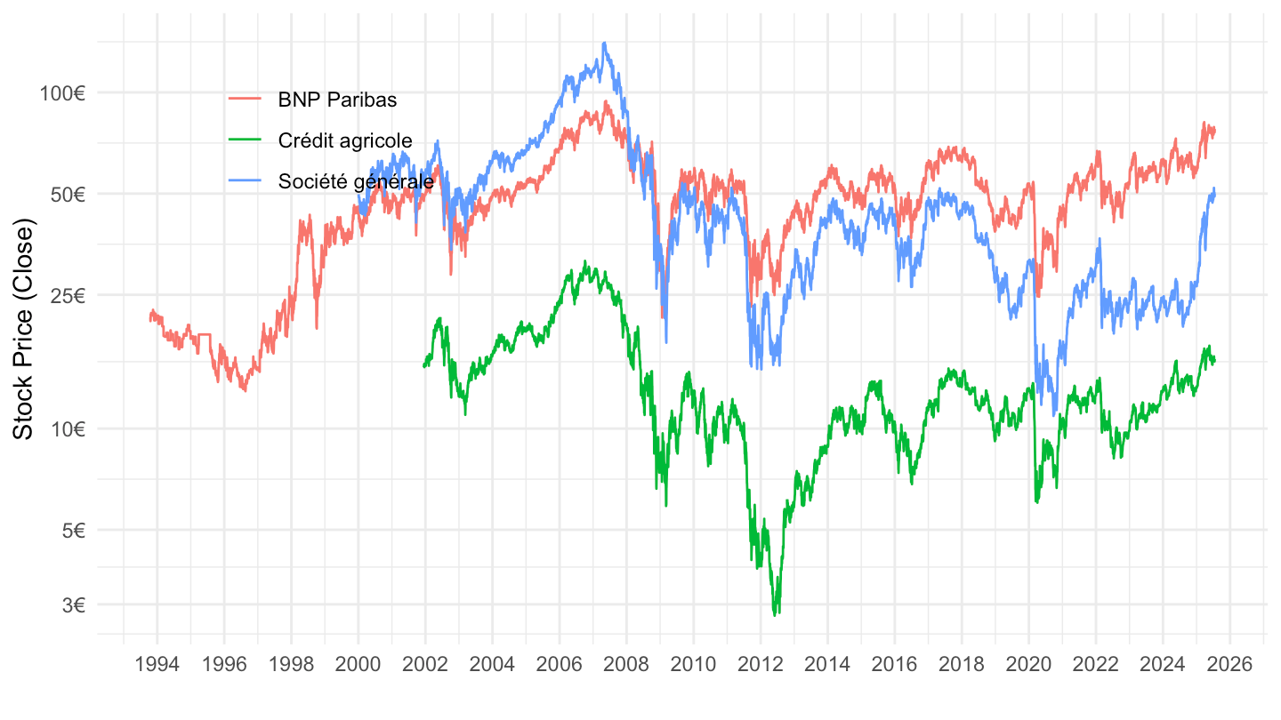
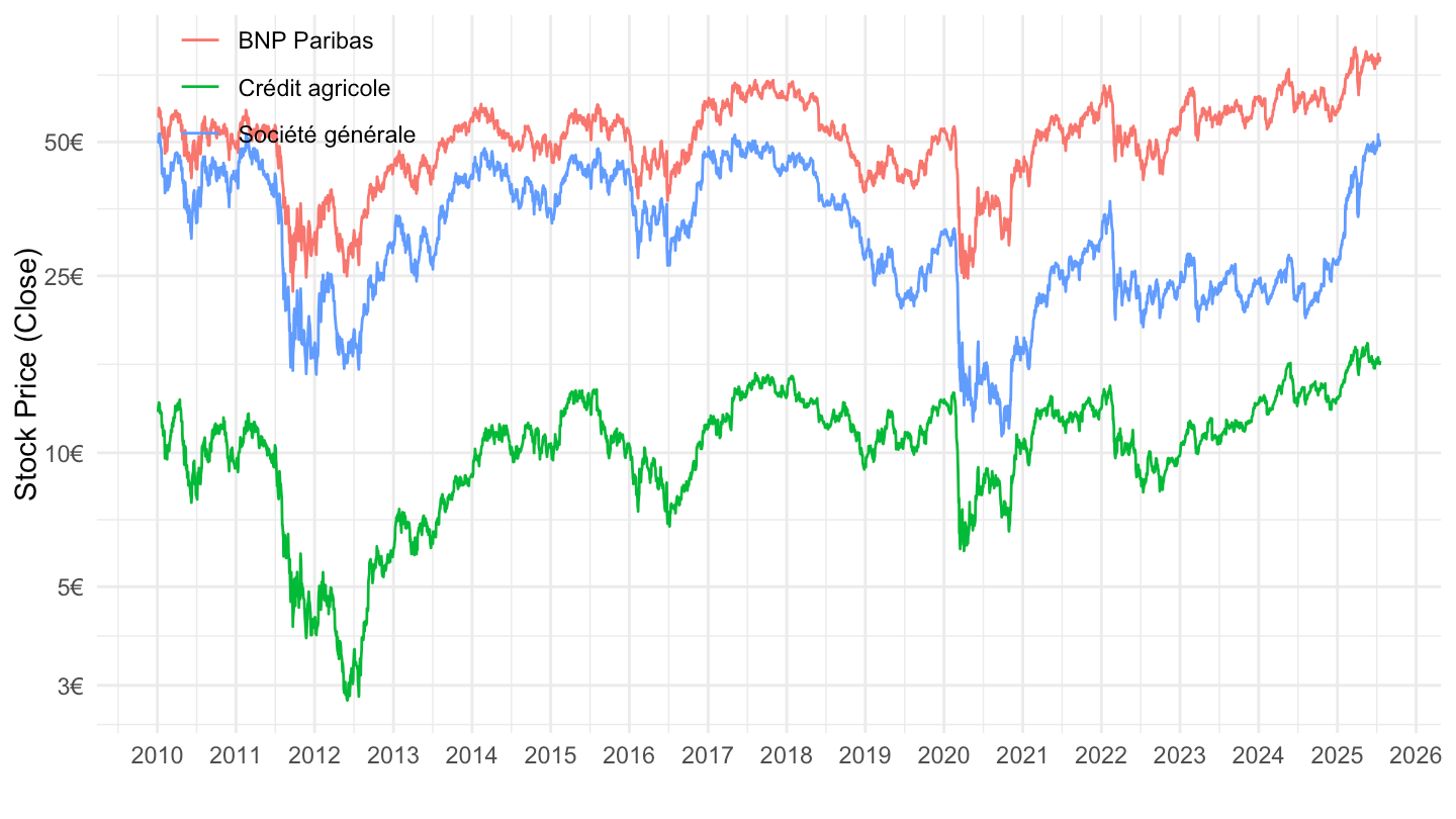
2010-
Code
CAC40 %>%
  left_join(CAC40_components, by = "symbol") %>%
  filter(symbol %in% c("BNP", "ACA", "GLE")) %>%
  filter(date >= as.Date("2010-01-01")) %>%
  ggplot + geom_line(aes(x = date, y = close, color = Symbol)) +
  theme_minimal() + xlab("") + ylab("Stock Price (Close)") +
  scale_x_date(breaks = seq(1960, 2100, 1) %>% paste0("-01-01") %>% as.Date,
               labels = date_format("%Y")) +
  scale_y_log10(breaks = c(1, 2, 3, 5, 10, 25, 50, 100, 200, 500),
                     labels = dollar_format(prefix = "", suffix = "€", accuracy = 1)) +
  theme(legend.position = c(0.15, 0.90),
        legend.title = element_blank())