Last observation: 2025 (N = 115)
First observation: 1960 (N = 1)
Last data update: 09 oct. 2026, 23:25
Last compile: 09 oct. 2026, 23:42
| LAST_COMPILE |
|---|
| 2026-10-09 |
NY.ADJ.NNAT.GN.ZS |>
  bind_rows(NY.ADJ.ICTR.GN.ZS) |>
  filter(iso3c == "USA") |>
  year_to_date() |>
  select(iso3c, date, variable, value) |>
  mutate(Variable = case_when(variable == "NY.ADJ.NNAT.GN.ZS" ~ "Net Saving",
                                  variable == "NY.ADJ.ICTR.GN.ZS" ~ "Gross Saving"),
         value = value /100) |>
  ggplot() + theme_minimal() +
  geom_line(aes(x = date, y = value, color = Variable, linetype = Variable)) +
  scale_color_manual(values = viridis(3)[1:2]) +
  theme(legend.title = element_blank(),
        legend.position = c(0.15, 0.15)) +
  geom_rect(data = nber_recessions |>
              filter(Peak > as.Date("1970-01-01")),
            aes(xmin = Peak, xmax = Trough, ymin = -Inf, ymax = +Inf),
            fill = 'grey', alpha = 0.5) +
  scale_x_date(breaks = nber_recessions$Peak,
               labels = date_format("%Y")) +
  scale_y_continuous(breaks = 0.01*seq(-2, 25, 2),
                     labels = scales::percent_format(accuracy = 1)) +
  xlab("") + ylab("% of GNI")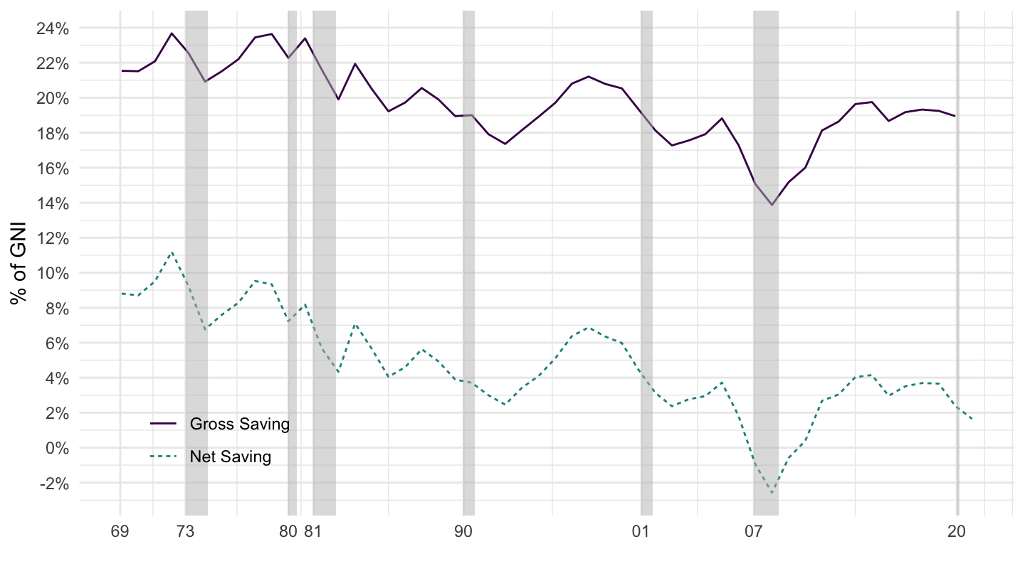
NY.ADJ.NNAT.GN.ZS |>
  bind_rows(NY.ADJ.ICTR.GN.ZS) |>
  filter(iso3c == "CHN") |>
  year_to_date() |>
  select(iso3c, date, variable, value) |>
  mutate(Variable = case_when(variable == "NY.ADJ.NNAT.GN.ZS" ~ "Net Saving",
                                  variable == "NY.ADJ.ICTR.GN.ZS" ~ "Gross Saving"),
         value = value /100) |>
  ggplot() + theme_minimal() +
  geom_line(aes(x = date, y = value, color = Variable, linetype = Variable)) +
  scale_color_manual(values = viridis(3)[1:2]) +
  theme(legend.title = element_blank(),
        legend.position = c(0.15, 0.75)) +
  geom_rect(data = nber_recessions |>
              filter(Peak > as.Date("1970-01-01")),
            aes(xmin = Peak, xmax = Trough, ymin = -Inf, ymax = +Inf),
            fill = 'grey', alpha = 0.5) +
  scale_x_date(breaks = nber_recessions$Peak,
               labels = date_format("%Y")) +
  scale_y_continuous(breaks = 0.01*seq(-2, 70, 2),
                     labels = scales::percent_format(accuracy = 1)) +
  xlab("") + ylab("% of GNI")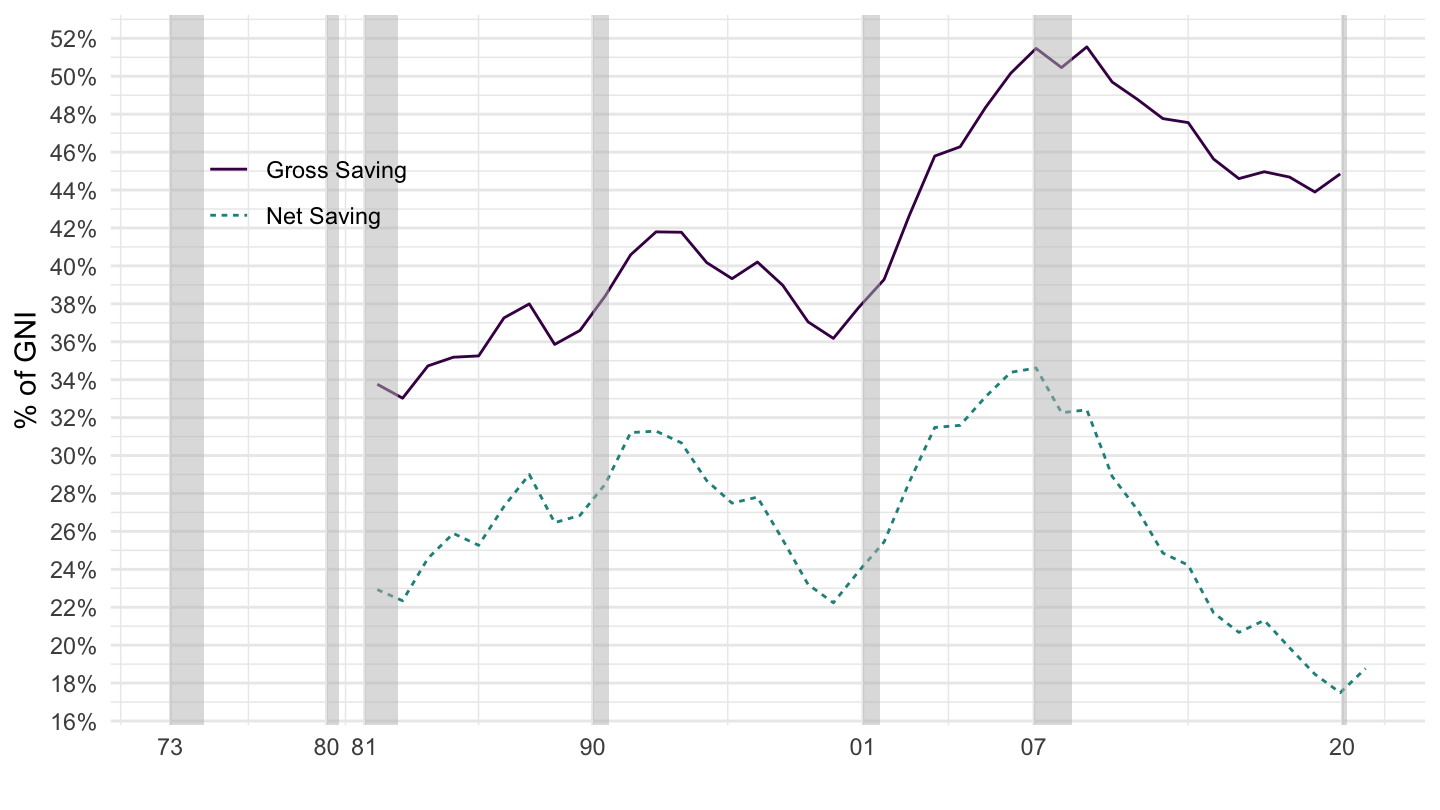
NY.GNS.ICTR.ZS |>
  bind_rows(NE.GDI.TOTL.ZS) |>
  filter(iso3c == "USA") |>
  year_to_date() |>
  select(iso3c, date, variable, value) |>
  mutate(Variable = case_when(variable == "NY.GNS.ICTR.ZS" ~ "Gross Saving",
                                  variable == "NE.GDI.TOTL.ZS" ~ "Gross Investment"),
         value = value /100) |>
  ggplot() + theme_minimal() +
  geom_line(aes(x = date, y = value, color = Variable, linetype = Variable)) +
  theme_minimal() +
  scale_color_manual(values = viridis(3)[1:2]) +
  theme(legend.title = element_blank(),
        legend.position = c(0.15, 0.15)) +
  geom_rect(data = nber_recessions |>
              filter(Peak > as.Date("1970-01-01")),
            aes(xmin = Peak, xmax = Trough, ymin = -Inf, ymax = +Inf),
            fill = 'grey', alpha = 0.5) +
  scale_x_date(breaks = nber_recessions$Peak,
               labels = date_format("%Y")) +
  scale_y_continuous(breaks = 0.01*seq(-2, 25, 2),
                     labels = scales::percent_format(accuracy = 1)) +
  xlab("") + ylab("% of GNI")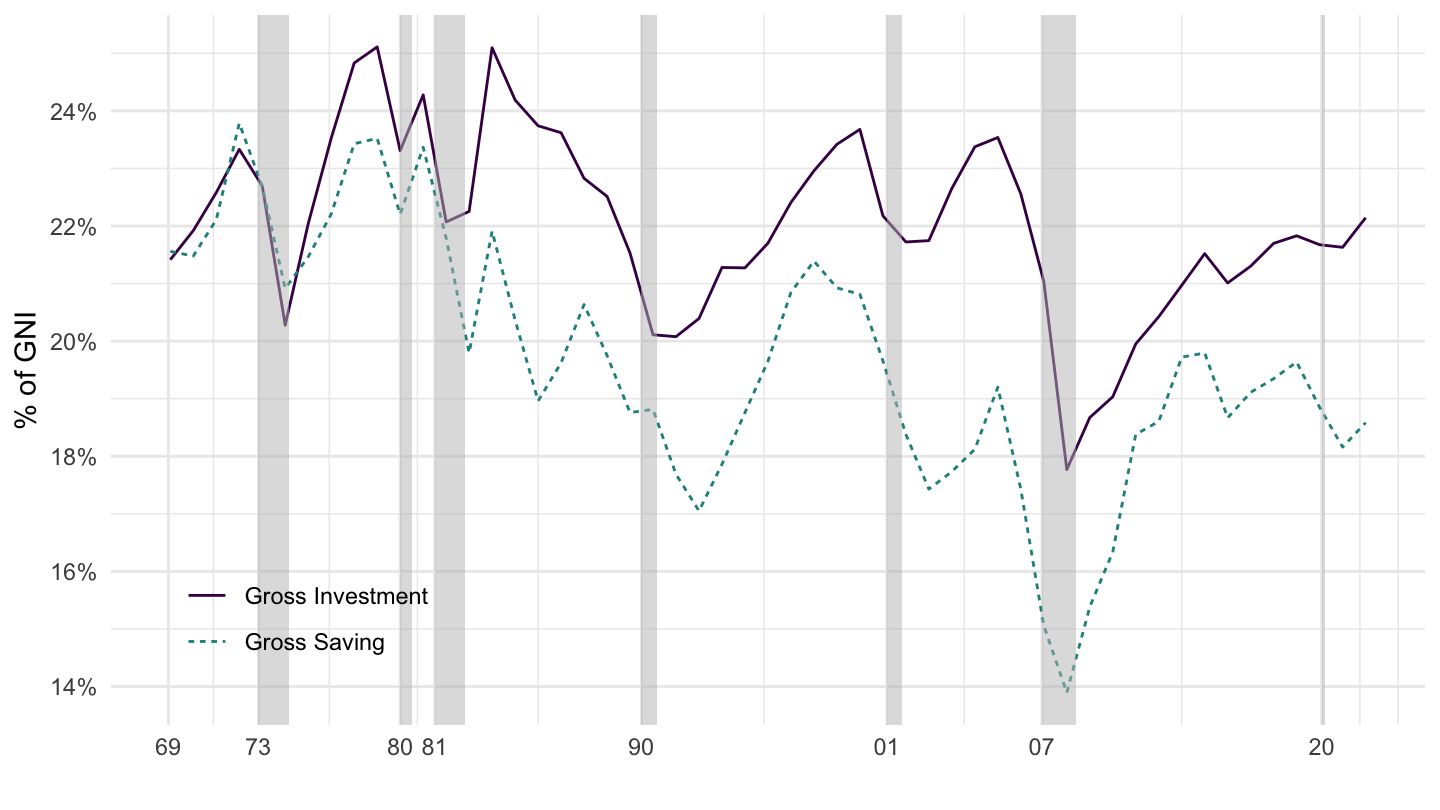
NY.GNS.ICTR.ZS |>
  bind_rows(NE.GDI.TOTL.ZS) |>
  filter(iso3c == "CHN") |>
  year_to_date() |>
  select(iso3c, date, variable, value) |>
  mutate(Variable = case_when(variable == "NY.GNS.ICTR.ZS" ~ "Gross Saving",
                                  variable == "NE.GDI.TOTL.ZS" ~ "Gross Investment"),
         value = value /100) |>
  ggplot() + theme_minimal() +
  geom_line(aes(x = date, y = value, color = Variable, linetype = Variable)) +
  theme_minimal() +
  scale_color_manual(values = viridis(3)[1:2]) +
  theme(legend.title = element_blank(),
        legend.position = c(0.15, 0.85)) +
  geom_rect(data = nber_recessions |>
              filter(Peak > as.Date("1970-01-01")),
            aes(xmin = Peak, xmax = Trough, ymin = -Inf, ymax = +Inf),
            fill = 'grey', alpha = 0.5) +
  scale_x_date(breaks = nber_recessions$Peak,
               labels = date_format("%Y")) +
  scale_y_continuous(breaks = 0.01*seq(-2, 80, 2),
                     labels = scales::percent_format(accuracy = 1)) +
  xlab("") + ylab("% of GNI")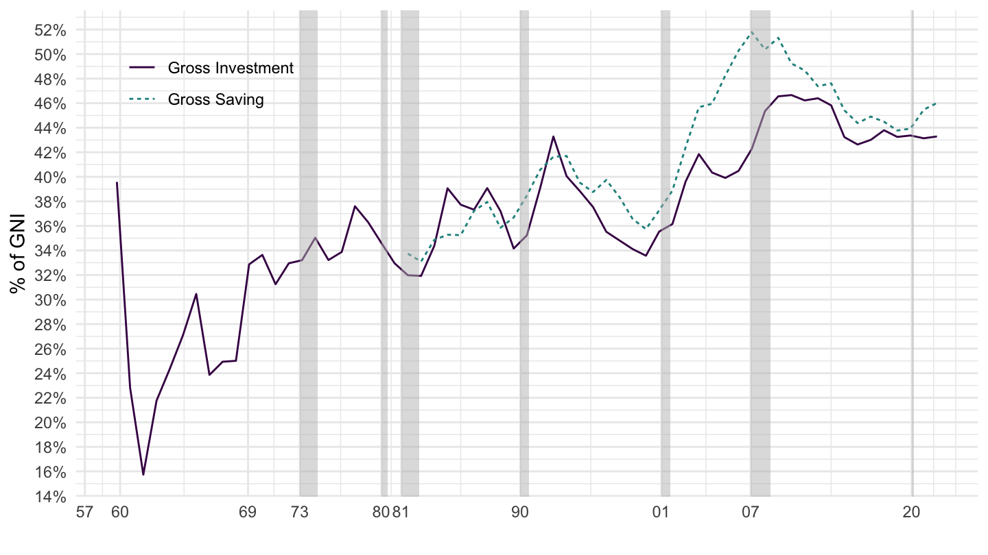
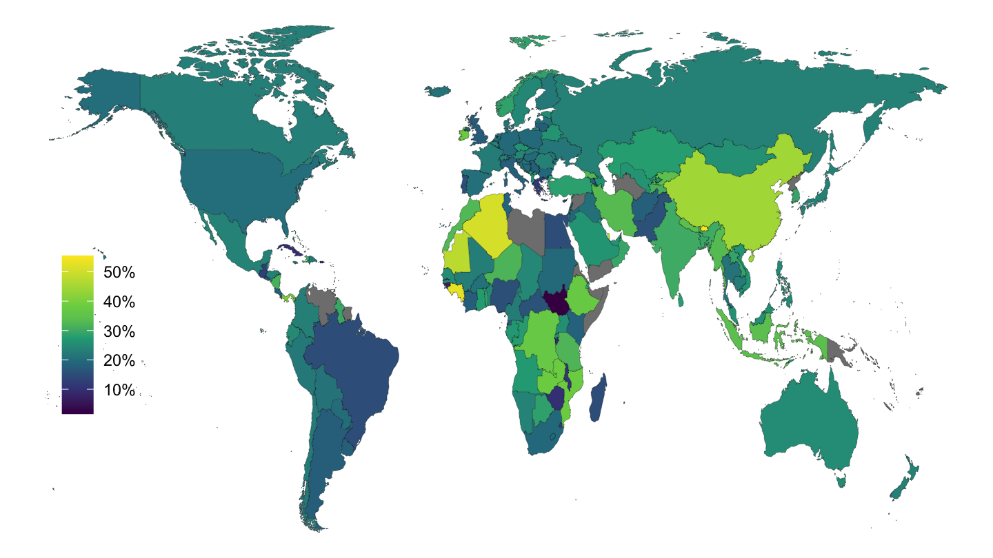
(ref:sav-gdp) Gross Saving (% of GDP), 2016.
WDI_api |>
  filter(year == 2016) |>
  filter(iso3c != "LBR", iso3c != "SLE") |>
  left_join(world, by = "iso2c") |>
  ggplot(aes(long, lat, group = group)) + theme_void() +
  geom_polygon(aes(fill = NY.GNS.ICTR.ZS/100), colour = alpha("black", 1/2), size = 0.1)  +
  scale_fill_viridis_c(labels = scales::percent_format(accuracy = 1),
                       breaks = seq(0, 0.6, 0.1),
                       values = c(0, 0.2, 0.4, 0.6, 1)) +
  theme(legend.position = c(0.1, 0.4),
        legend.title = element_blank())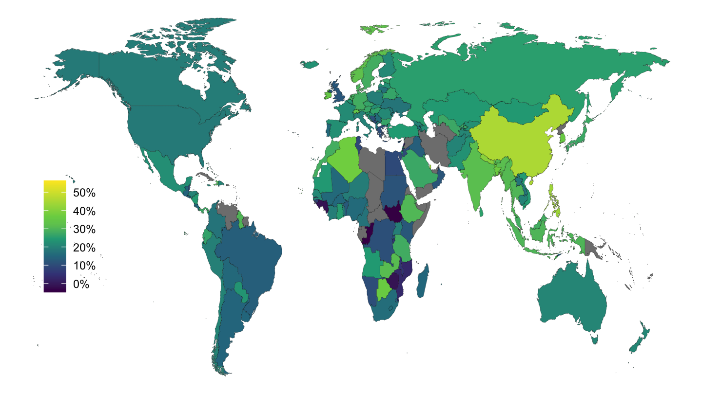
(ref:inv-gdp) Gross Investment (% of GDP), 2016.
WDI_api |>
  filter(year == 2016) |>
  filter(iso3c != "LBR", iso3c != "SLE") |>
  left_join(world, by = "iso2c") |>
  ggplot(aes(long, lat, group = group)) + theme_void() +
  geom_polygon(aes(fill = NE.GDI.TOTL.ZS/100), colour = alpha("black", 1/2), size = 0.1)  +
  scale_fill_viridis_c(labels = scales::percent_format(accuracy = 1),
                       breaks = seq(0, 0.6, 0.1),
                       values = c(0, 0.2, 0.4, 0.6, 1)) +
  theme(legend.position = c(0.1, 0.4),
        legend.title = element_blank())