Last observation: 2025 (N = 229)
First observation: 1991 (N = 234)
Last data update: 04 oct. 2026, 23:42
Last compile: 05 oct. 2026, 00:00
SL.UEM.TOTL.ZS |>
  left_join(iso2c, by = "iso2c") |>
  group_by(iso2c, Iso2c) |>
  mutate(value = round(value, 1)) |>
  summarise(Nobs = n(),
            `Year 1` = first(year),
            `Unemployment 1 (Bn)` = first(value),
            `Year 2` = last(year),
            `Unemployment 2 (Bn)` = last(value)) |>
  arrange(-Nobs) %>%
{if (is_html_output()) datatable(., filter = 'top', rownames = F) else .}data |>
left_join(INDICATOR) |>
year_to_date() |>
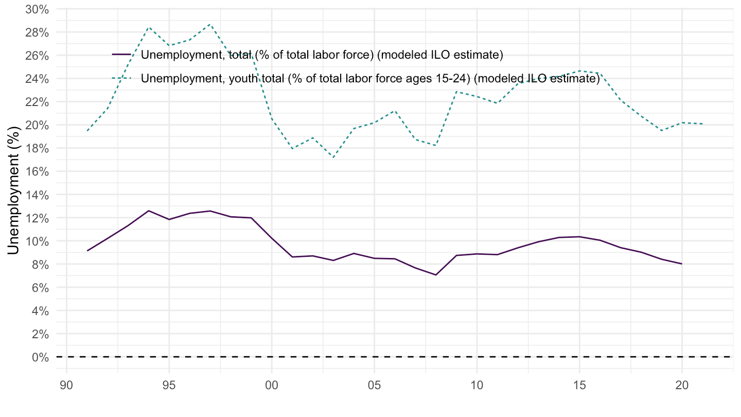
filter(iso2c == "TR") |>
ggplot() + theme_minimal() + xlab("") + ylab("Unemployment (%)") +
geom_line(aes(x = date, y = value/100, linetype = Indicator, color = Indicator)) +
theme(legend.title = element_blank(),
legend.position = c(0.65, 0.85)) +
scale_x_date(breaks = seq(1900, 2100, 5) |> paste0("-01-01") |> as.Date(),
labels = date_format("%Y")) +
scale_y_continuous(breaks = 0.01*seq(-100, 10000, 2),
labels = percent_format(a = 1)) +
geom_hline(yintercept = 0, linetype = "dashed", color = "black")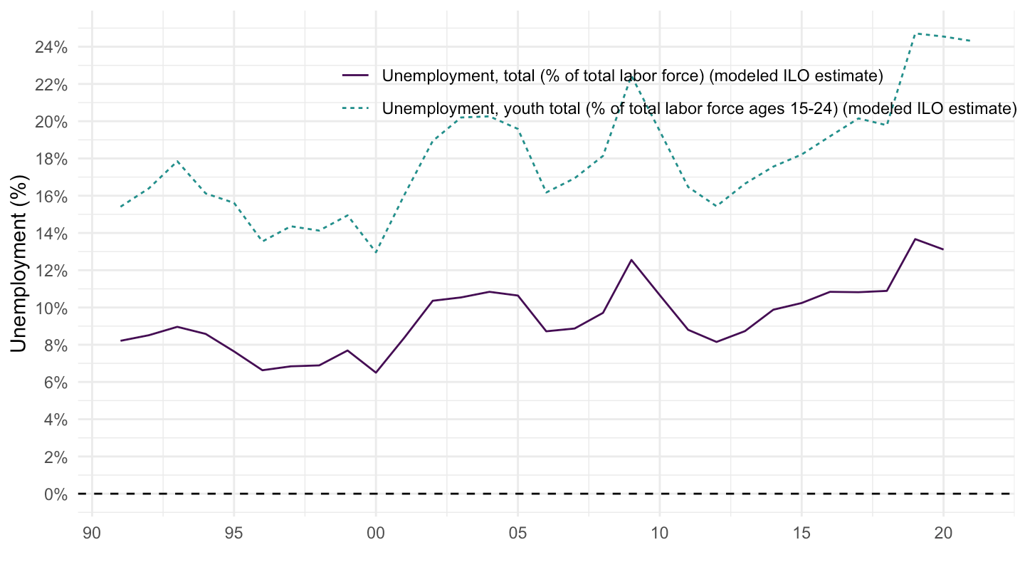
data |>
  left_join(INDICATOR) |>
  year_to_date() |>
  filter(iso2c == "TR") |>
  filter(date >= as.Date("1995-01-01"),
         date <= as.Date("2005-01-01")) |>
  ggplot() + theme_minimal() + xlab("") + ylab("Unemployment (%)") +
  geom_line(aes(x = date, y = value/100, linetype = Indicator, color = Indicator)) +

  theme(legend.title = element_blank(),
        legend.position = c(0.4, 0.2)) +
  scale_x_date(breaks = seq(1900, 2100, 2) |> paste0("-01-01") |> as.Date(),
               labels = date_format("%Y")) +
  scale_y_continuous(breaks = 0.01*seq(-100, 10000, 2),
                     labels = percent_format(a = 1)) +
  geom_hline(yintercept = 0, linetype = "dashed", color = "black")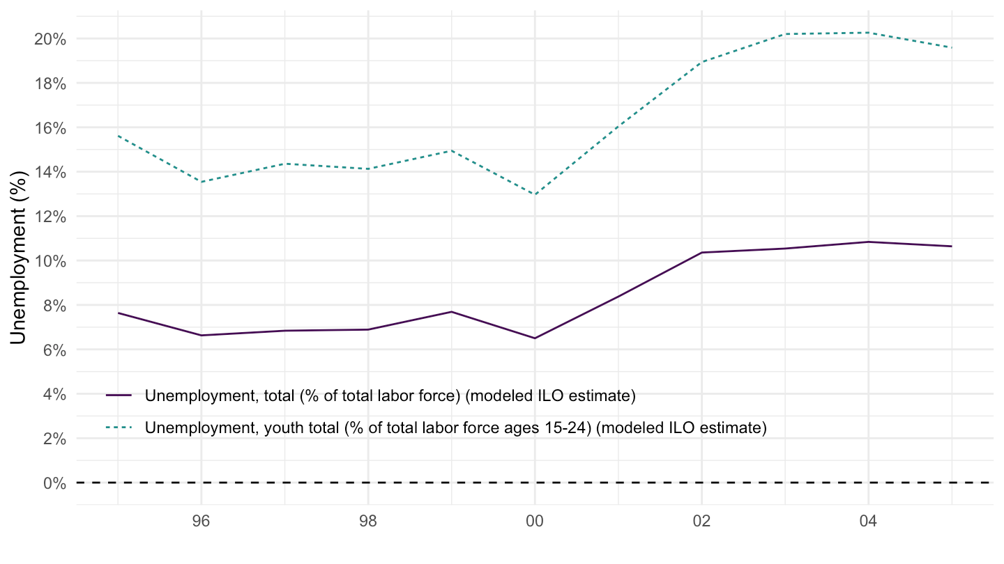
data |>
  left_join(INDICATOR) |>
  year_to_date() |>
  filter(iso2c == "HK") |>
  ggplot() + theme_minimal() + xlab("") + ylab("Unemployment (%)") +
  geom_line(aes(x = date, y = value/100, linetype = Indicator, color = Indicator)) +

  theme(legend.title = element_blank(),
        legend.position = c(0.65, 0.85)) +
  scale_x_date(breaks = seq(1900, 2100, 5) |> paste0("-01-01") |> as.Date(),
               labels = date_format("%Y")) +
  scale_y_continuous(breaks = 0.01*seq(-100, 10000, 2),
                     labels = percent_format(a = 1)) +
  geom_hline(yintercept = 0, linetype = "dashed", color = "black")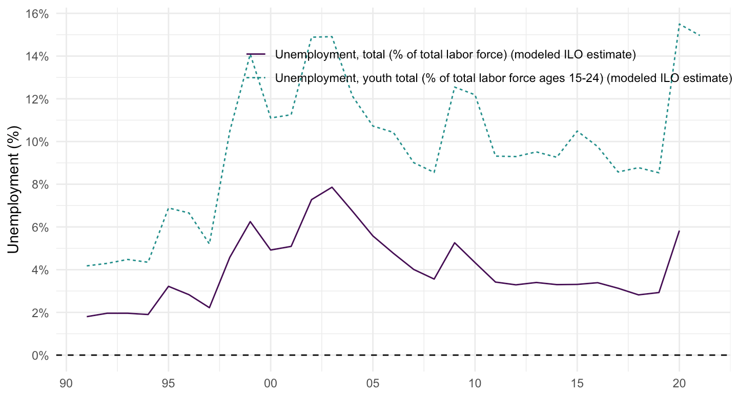
data |>
  left_join(INDICATOR) |>
  year_to_date() |>
  filter(iso2c == "HK",
         date >= as.Date("1993-01-01")) |>
  ggplot() + theme_minimal() + xlab("") + ylab("Unemployment (%)") +
  geom_line(aes(x = date, y = value/100, linetype = Indicator, color = Indicator)) +

  theme(legend.title = element_blank(),
        legend.position = c(0.65, 0.85)) +
  scale_x_date(breaks = seq(1900, 2100, 2) |> paste0("-01-01") |> as.Date(),
               labels = date_format("%Y")) +
  scale_y_continuous(breaks = 0.01*seq(-100, 10000, 2),
                     labels = percent_format(a = 1)) +
  geom_hline(yintercept = 0, linetype = "dashed", color = "black")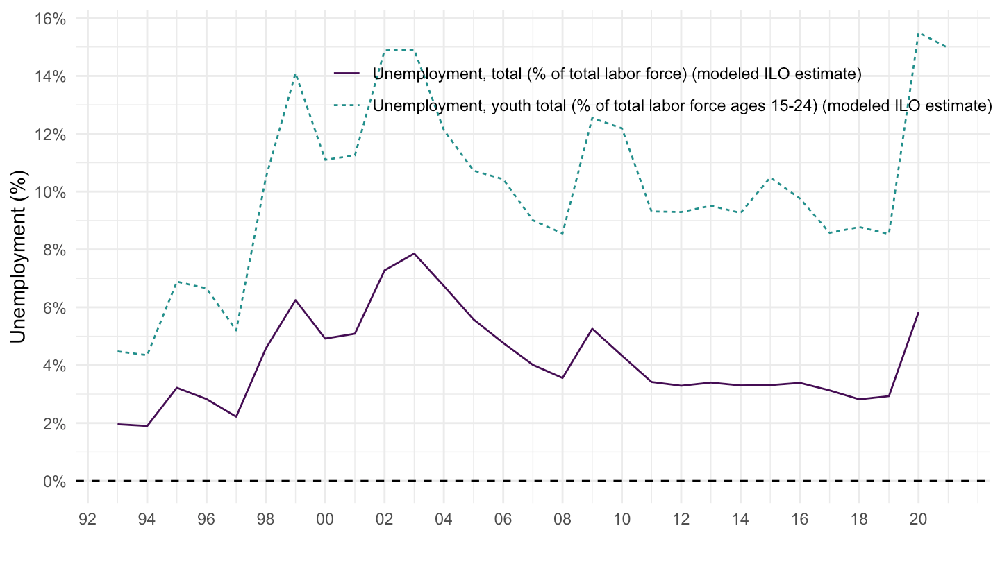
data |>
  left_join(INDICATOR) |>
  year_to_date() |>
  filter(iso2c == "IS") |>
  ggplot() + theme_minimal() + xlab("") + ylab("Unemployment (%)") +
  geom_line(aes(x = date, y = value/100, linetype = Indicator, color = Indicator)) +

  theme(legend.title = element_blank(),
        legend.position = c(0.45, 0.85)) +
  scale_x_date(breaks = seq(1900, 2100, 5) |> paste0("-01-01") |> as.Date(),
               labels = date_format("%Y")) +
  scale_y_continuous(breaks = 0.01*seq(-100, 10000, 2),
                     labels = percent_format(a = 1)) +
  geom_hline(yintercept = 0, linetype = "dashed", color = "black")
data |>
  left_join(INDICATOR) |>
  year_to_date() |>
  filter(iso2c == "IS",
         date >= as.Date("1993-01-01")) |>
  ggplot() + theme_minimal() + xlab("") + ylab("Unemployment (%)") +
  geom_line(aes(x = date, y = value/100, linetype = Indicator, color = Indicator)) +

  theme(legend.title = element_blank(),
        legend.position = c(0.45, 0.85)) +
  scale_x_date(breaks = seq(1900, 2100, 2) |> paste0("-01-01") |> as.Date(),
               labels = date_format("%Y")) +
  scale_y_continuous(breaks = 0.01*seq(-100, 10000, 2),
                     labels = percent_format(a = 1)) +
  geom_hline(yintercept = 0, linetype = "dashed", color = "black")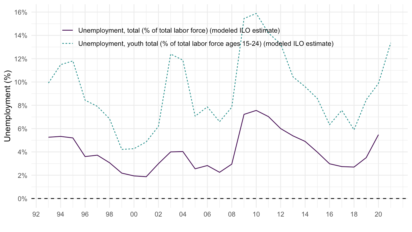
SL.UEM.TOTL.ZS |>
  filter(iso2c %in% c("FR", "DE", "IT")) |>
  left_join(iso2c, by = "iso2c") |>
  add_flag_color("Iso2c") |>
  year_to_date() |>
  mutate(value = value/100) |>
  ggplot() + geom_line(aes(x = date, y = value, color = color)) + theme_minimal() +
  xlab("") + ylab("Unemployment, Total (% of labor force)") +
  scale_color_identity() + add_flags +
  scale_x_date(breaks = seq(1900, 2100, 5) |> paste0("-01-01") |> as.Date(),
               labels = date_format("%Y")) +
  scale_y_continuous(breaks = 0.01*seq(-100, 10000, 2),
                     labels = percent_format(a = 1)) +
  geom_hline(yintercept = 0, linetype = "dashed", color = "grey")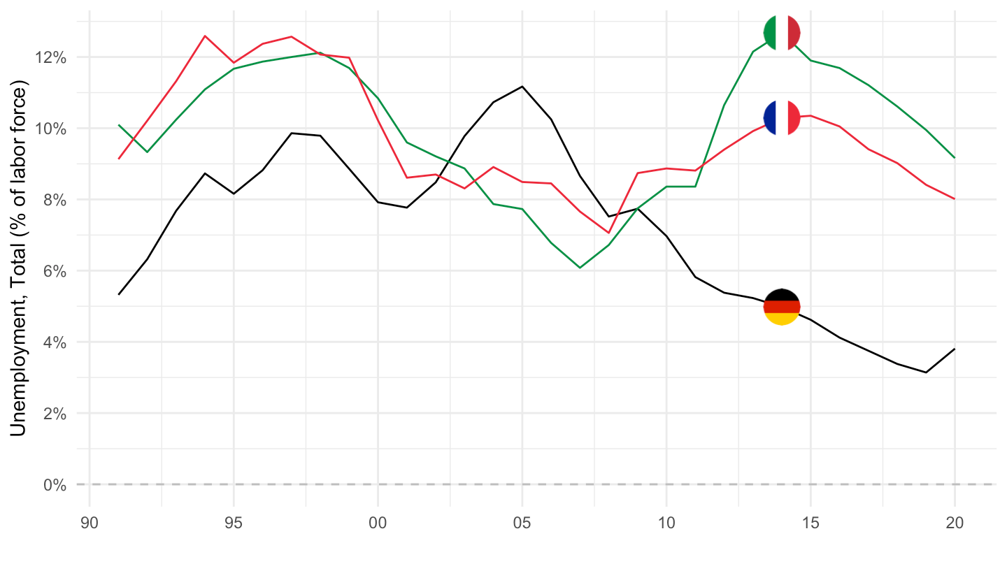
SL.UEM.TOTL.ZS |>
  year_to_date() |>
  filter(iso2c %in% c("SG", "PH", "ID"),
         date >= as.Date("1990-01-01"),
         date <= as.Date("2005-01-01")) |>
  left_join(iso2c, by = "iso2c") |>
  ggplot() + geom_line() + theme_minimal() +
  aes(x = date, y = value/100, color = Iso2c, linetype = Iso2c) +
  xlab("") + ylab("Unemployment, Total (% of labor force)") +
  scale_color_manual(values = viridis(4)[1:3]) +
  theme(legend.title = element_blank(),
        legend.position = c(0.85, 0.85)) +
  scale_x_date(breaks = seq(1900, 2100, 1) |> paste0("-01-01") |> as.Date(),
               labels = date_format("%Y")) +
  scale_y_continuous(breaks = 0.01*seq(-100, 10000, 1),
                     labels = percent_format(a = 1)) +
  geom_hline(yintercept = 0, linetype = "dashed", color = "grey")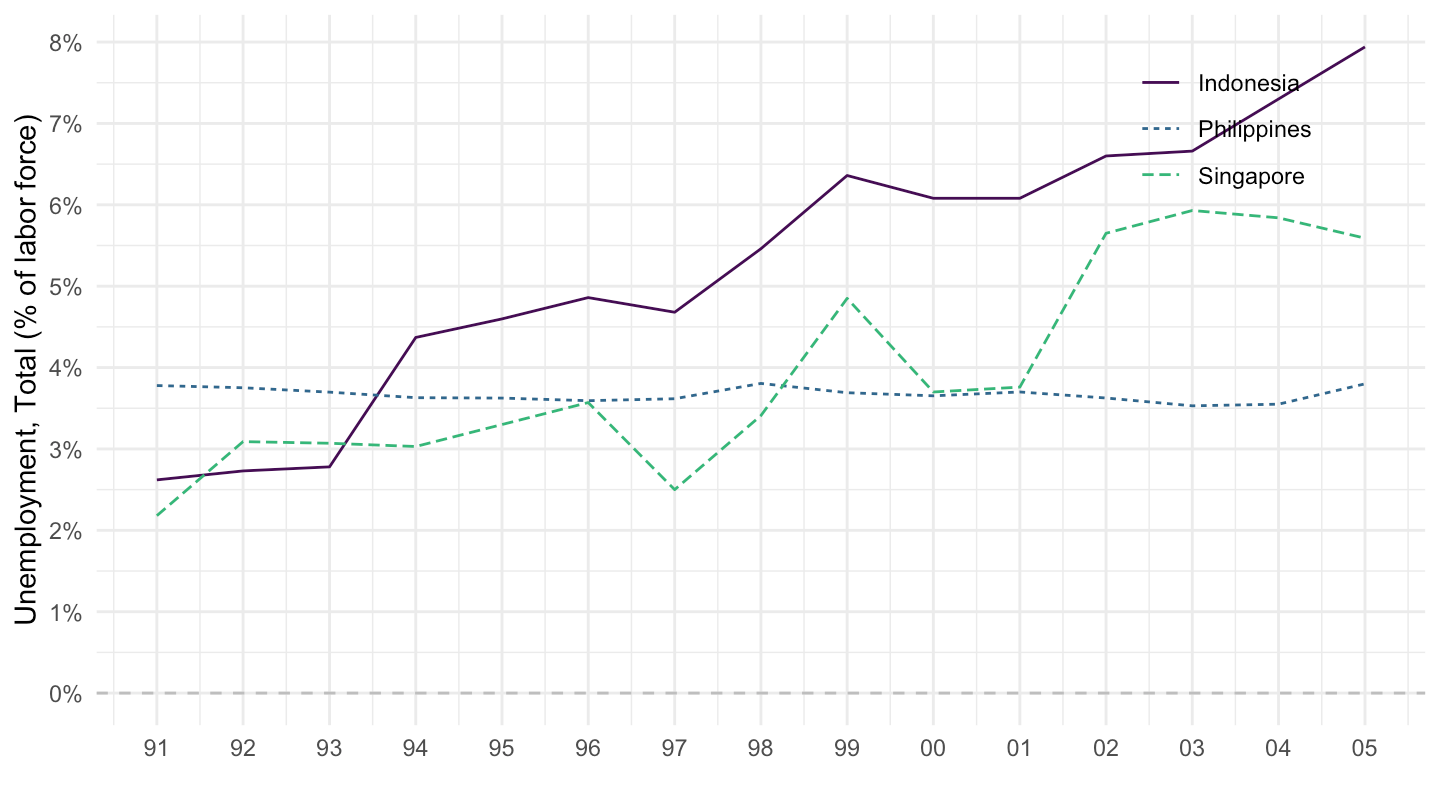
SL.UEM.TOTL.ZS |>
  year_to_date() |>
  filter(iso2c %in% c("TH", "MY", "KR"),
         date >= as.Date("1990-01-01"),
         date <= as.Date("2005-01-01")) |>
  left_join(iso2c, by = "iso2c") |>
  ggplot() + geom_line() + theme_minimal() +
  aes(x = date, y = value/100, color = Iso2c, linetype = Iso2c) +
  xlab("") + ylab("Unemployment, Total (% of labor force)") +
  scale_color_manual(values = viridis(4)[1:3]) +
  theme(legend.title = element_blank(),
        legend.position = c(0.85, 0.85)) +
  scale_x_date(breaks = seq(1900, 2100, 1) |> paste0("-01-01") |> as.Date(),
               labels = date_format("%Y")) +
  scale_y_continuous(breaks = 0.01*seq(-100, 10000, 1),
                     labels = percent_format(a = 1)) +
  geom_hline(yintercept = 0, linetype = "dashed", color = "grey")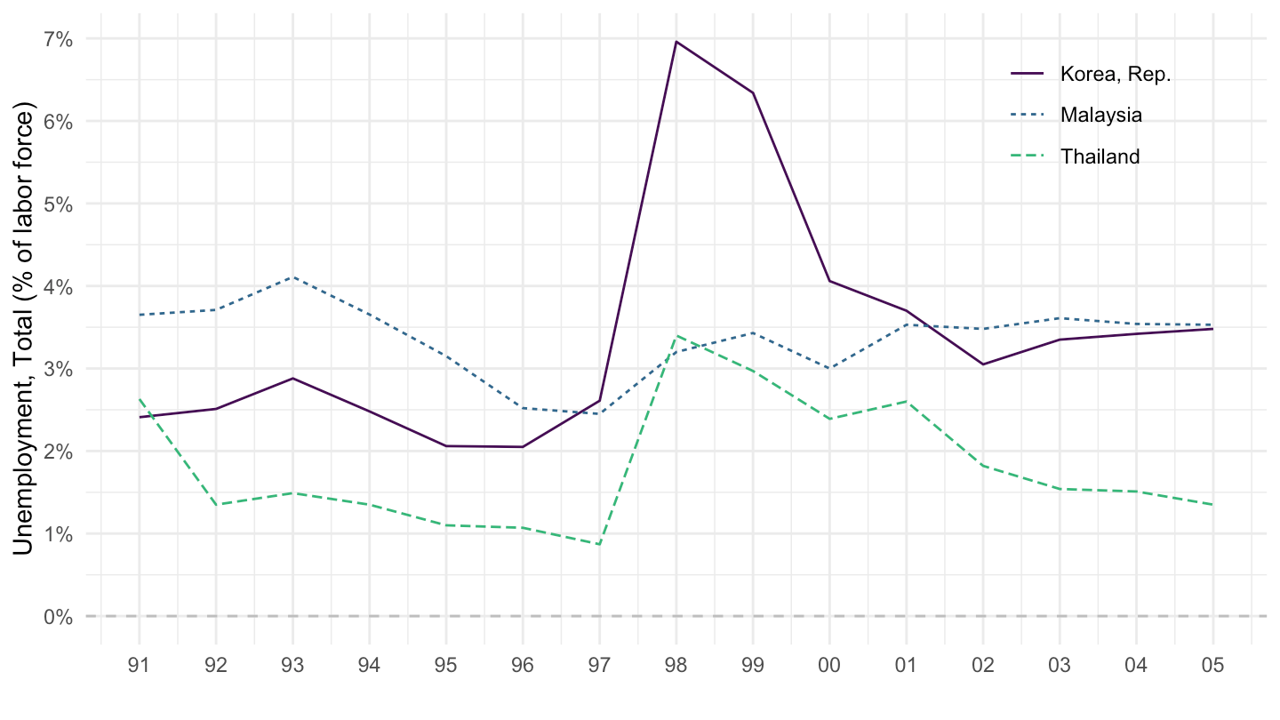
SL.UEM.TOTL.ZS |>
  filter(iso2c %in% c("DK", "SE", "NL")) |>
  left_join(iso2c, by = "iso2c") |>
  add_flag_color("Iso2c") |>
  year_to_date() |>
  mutate(value = value/100) |>
  ggplot() + geom_line(aes(x = date, y = value, color = color)) + theme_minimal() +
  xlab("") + ylab("Unemployment, Total (% of labor force)") +
  scale_color_identity() + add_flags +
  scale_x_date(breaks = seq(1900, 2100, 5) |> paste0("-01-01") |> as.Date(),
               labels = date_format("%Y")) +
  scale_y_continuous(breaks = 0.01*seq(-100, 10000, 2),
                     labels = percent_format(a = 1)) +
  geom_hline(yintercept = 0, linetype = "dashed", color = "grey")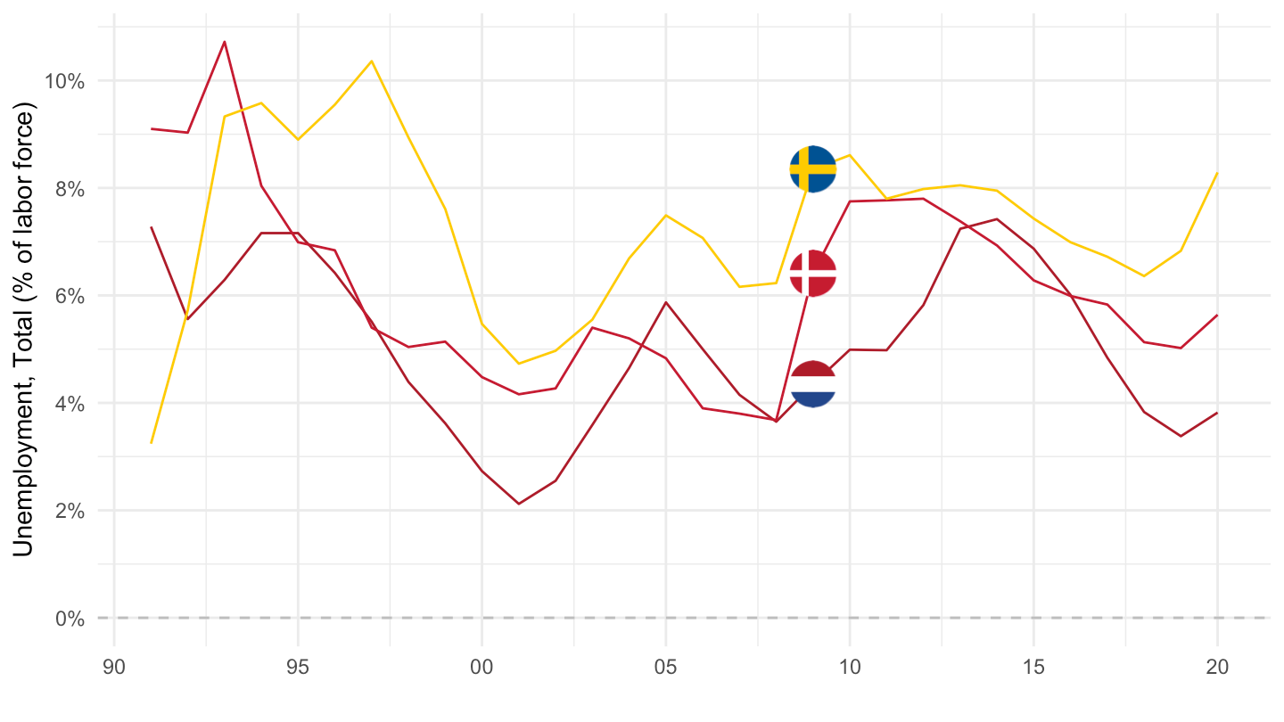
SL.UEM.TOTL.ZS |>
  filter(iso2c %in% c("JP", "US", "GB")) |>
  left_join(iso2c, by = "iso2c") |>
  add_flag_color("Iso2c") |>
  year_to_date() |>
  mutate(value = value/100) |>
  ggplot() + geom_line(aes(x = date, y = value, color = color)) + theme_minimal() +
  xlab("") + ylab("Unemployment, Total (% of labor force)") +
  scale_color_identity() + add_flags +
  scale_x_date(breaks = seq(1900, 2100, 5) |> paste0("-01-01") |> as.Date(),
               labels = date_format("%Y")) +
  scale_y_continuous(breaks = 0.01*seq(-100, 10000, 2),
                     labels = percent_format(a = 1)) +
  geom_hline(yintercept = 0, linetype = "dashed", color = "grey")
data |>
  left_join(INDICATOR) |>
  year_to_date() |>
  filter(iso2c == "IT") |>
  ggplot() + theme_minimal() + xlab("") + ylab("Unemployment (%)") +
  geom_line(aes(x = date, y = value/100, linetype = Indicator, color = Indicator)) +

  theme(legend.title = element_blank(),
        legend.position = c(0.45, 0.85)) +
  scale_x_date(breaks = seq(1900, 2100, 5) |> paste0("-01-01") |> as.Date(),
               labels = date_format("%Y")) +
  scale_y_continuous(breaks = 0.01*seq(-100, 10000, 2),
                     labels = percent_format(a = 1)) +
  geom_hline(yintercept = 0, linetype = "dashed", color = "black")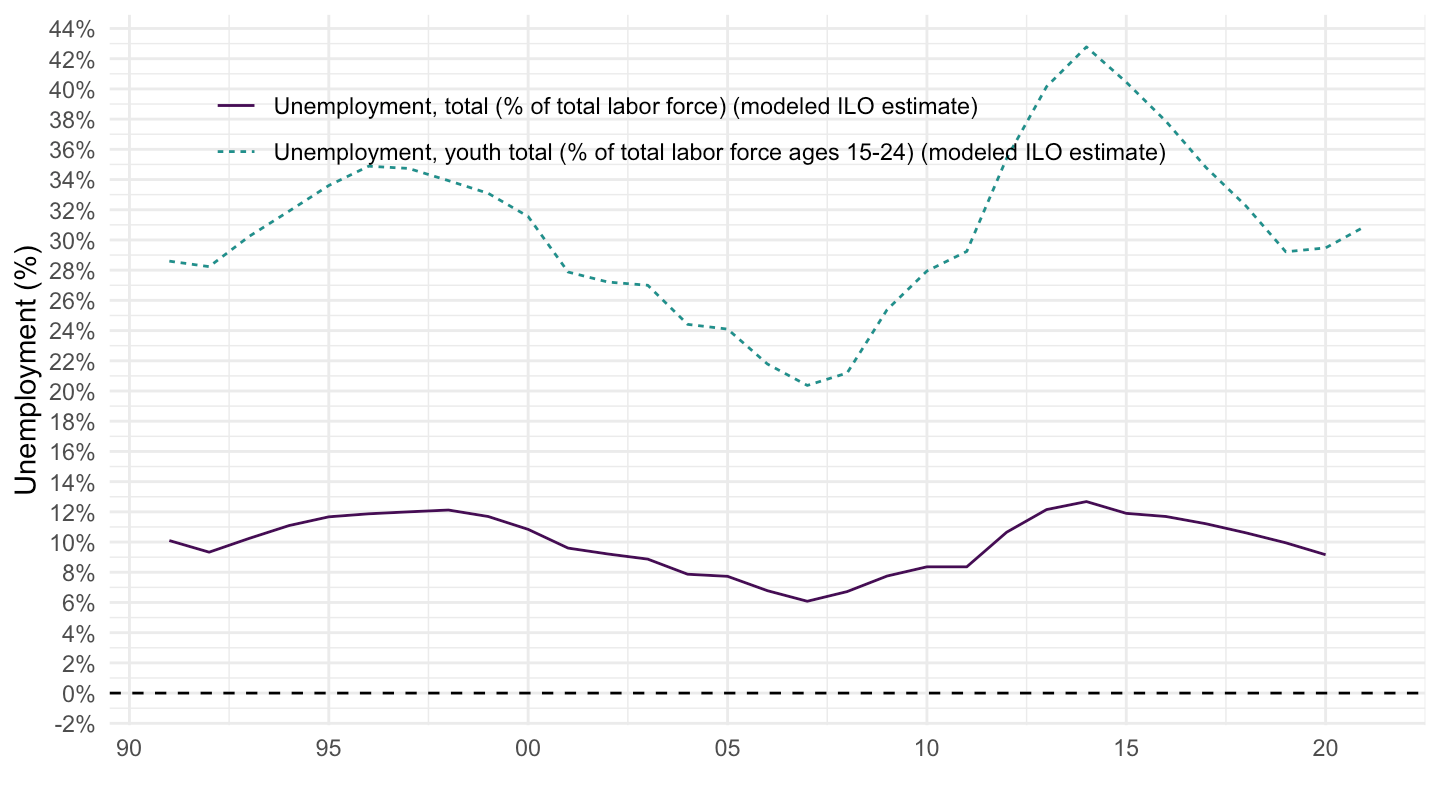
data |>
  left_join(INDICATOR) |>
  year_to_date() |>
  filter(iso2c == "IT",
         date >= as.Date("1995-01-01")) |>
  ggplot() + theme_minimal() + xlab("") + ylab("Unemployment (%)") +
  geom_line(aes(x = date, y = value/100, linetype = Indicator, color = Indicator)) +

  theme(legend.title = element_blank(),
        legend.position = c(0.45, 0.85)) +
  scale_x_date(breaks = seq(1900, 2100, 5) |> paste0("-01-01") |> as.Date(),
               labels = date_format("%Y")) +
  scale_y_continuous(breaks = 0.01*seq(-100, 10000, 2),
                     labels = percent_format(a = 1)) +
  geom_hline(yintercept = 0, linetype = "dashed", color = "black")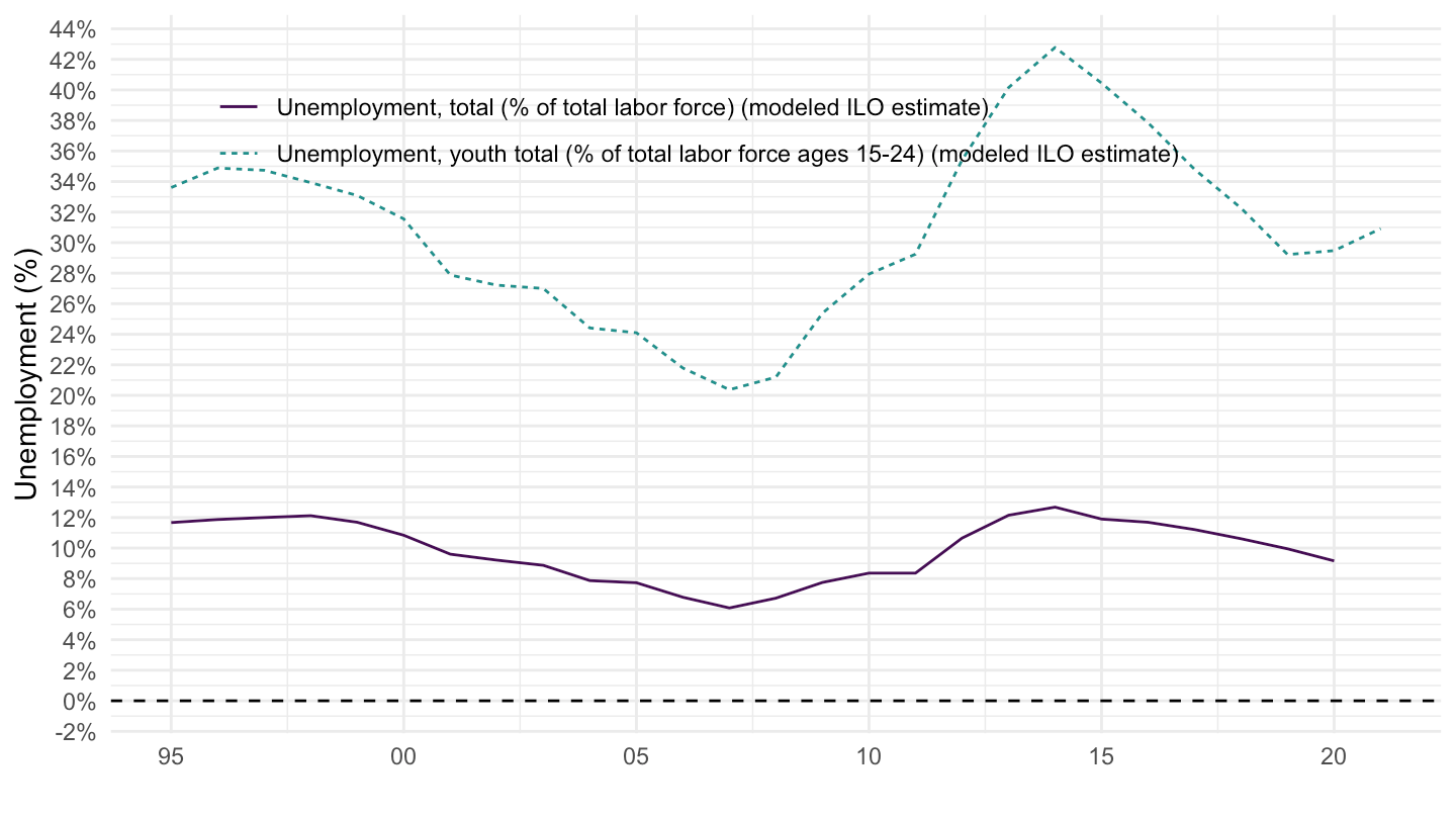
data |>
  left_join(INDICATOR) |>
  year_to_date() |>
  filter(iso2c == "AR") |>
  ggplot() + theme_minimal() + xlab("") + ylab("Unemployment (%)") +
  geom_line(aes(x = date, y = value/100, linetype = Indicator, color = Indicator)) +

  theme(legend.title = element_blank(),
        legend.position = c(0.45, 0.85)) +
  scale_x_date(breaks = seq(1900, 2100, 5) |> paste0("-01-01") |> as.Date(),
               labels = date_format("%Y")) +
  scale_y_continuous(breaks = 0.01*seq(-100, 10000, 2),
                     labels = percent_format(a = 1)) +
  geom_hline(yintercept = 0, linetype = "dashed", color = "black")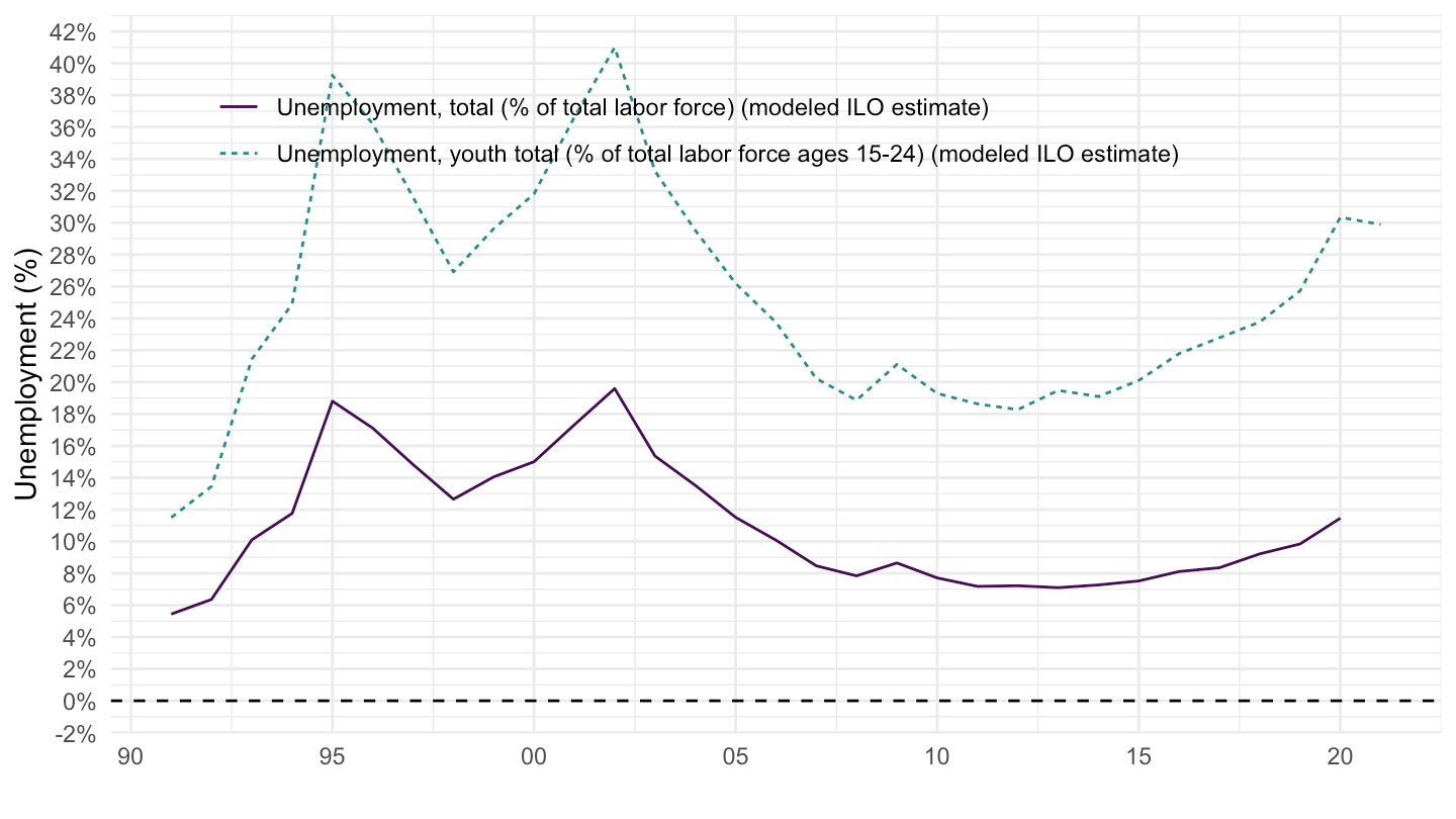
SL.UEM.TOTL.ZS |>
  year_to_date() |>
  filter(iso2c == "AR",
         date >= as.Date("1996-01-01"),
         date <= as.Date("2005-01-01")) |>
  ggplot() + geom_line() + theme_minimal() +
  aes(x = date, y = value/100) + xlab("") + ylab("Unemployment, Total (% of labor force)") +
  scale_x_date(breaks = seq(1900, 2100, 1) |> paste0("-01-01") |> as.Date(),
               labels = date_format("%Y")) +
  scale_y_continuous(breaks = 0.01*seq(-100, 10000, 5),
                     labels = percent_format(a = 1)) +
  geom_hline(yintercept = 0, linetype = "dashed", color = "grey")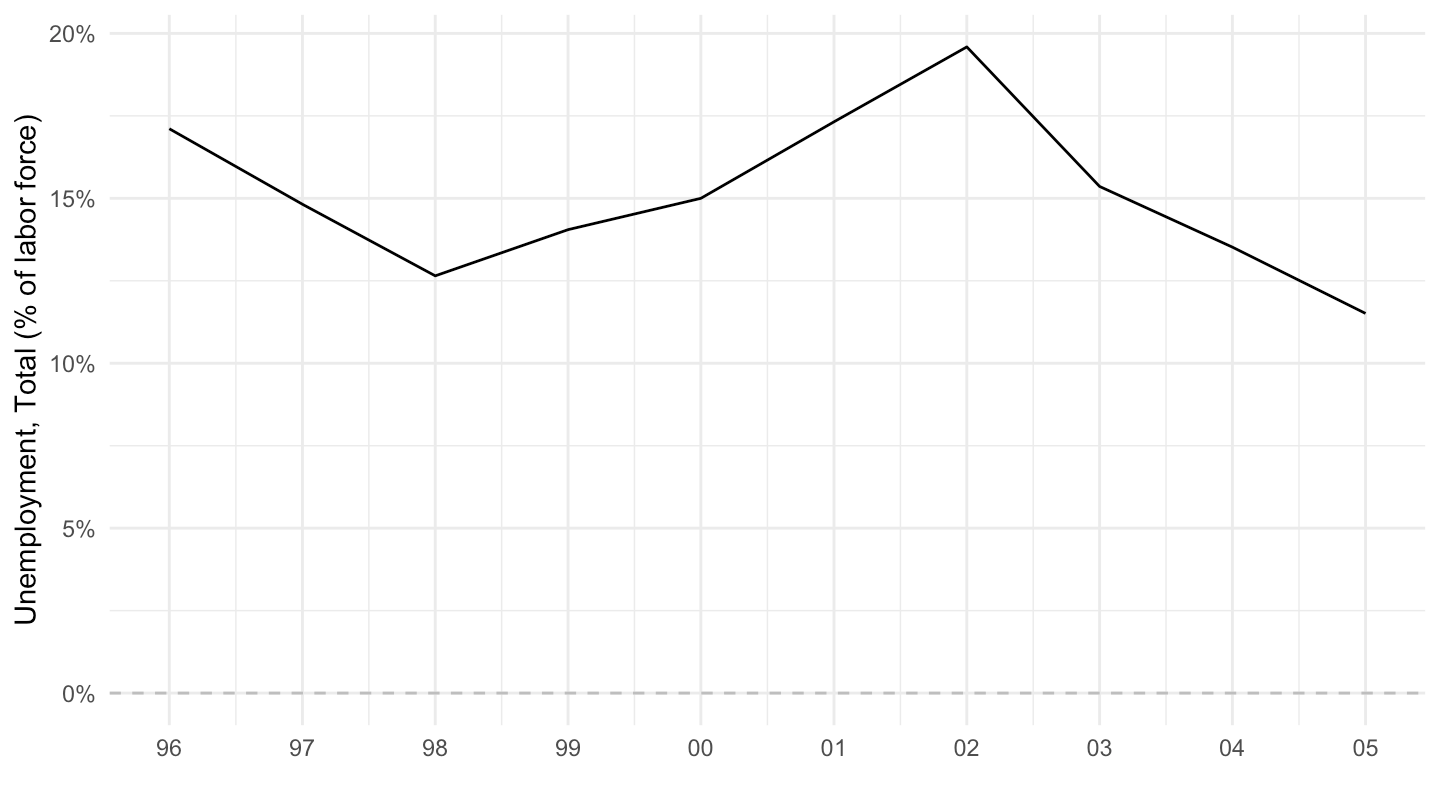
SL.UEM.TOTL.ZS |>
  year_to_date() |>
  filter(iso2c == "AR",
         date >= as.Date("1996-01-01"),
         date <= as.Date("2020-01-01")) |>
  ggplot() + geom_line() + theme_minimal() +
  aes(x = date, y = value/100) + xlab("") + ylab("Unemployment, Total (% of labor force)") +
  scale_x_date(breaks = seq(1900, 2100, 1) |> paste0("-01-01") |> as.Date(),
               labels = date_format("%Y")) +
  scale_y_continuous(breaks = 0.01*seq(-100, 10000, 5),
                     labels = percent_format(a = 1)) +
  geom_hline(yintercept = 0, linetype = "dashed", color = "grey")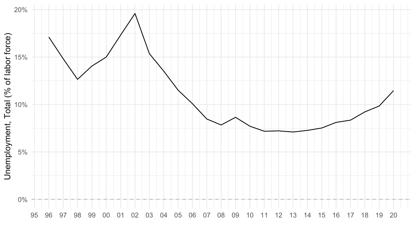
SL.UEM.TOTL.ZS |>
  filter(iso2c == "CN") |>
  year_to_date() |>
  ggplot() + geom_line() + theme_minimal() +
  aes(x = date, y = value/100) + xlab("") + ylab("Unemployment, Total (% of labor force)") +
  scale_x_date(breaks = seq(1900, 2100, 2) |> paste0("-01-01") |> as.Date(),
               labels = date_format("%Y")) +
  scale_y_continuous(breaks = 0.01*seq(-100, 10000, 1),
                     labels = percent_format(a = 1)) +
  geom_hline(yintercept = 0, linetype = "dashed", color = "grey")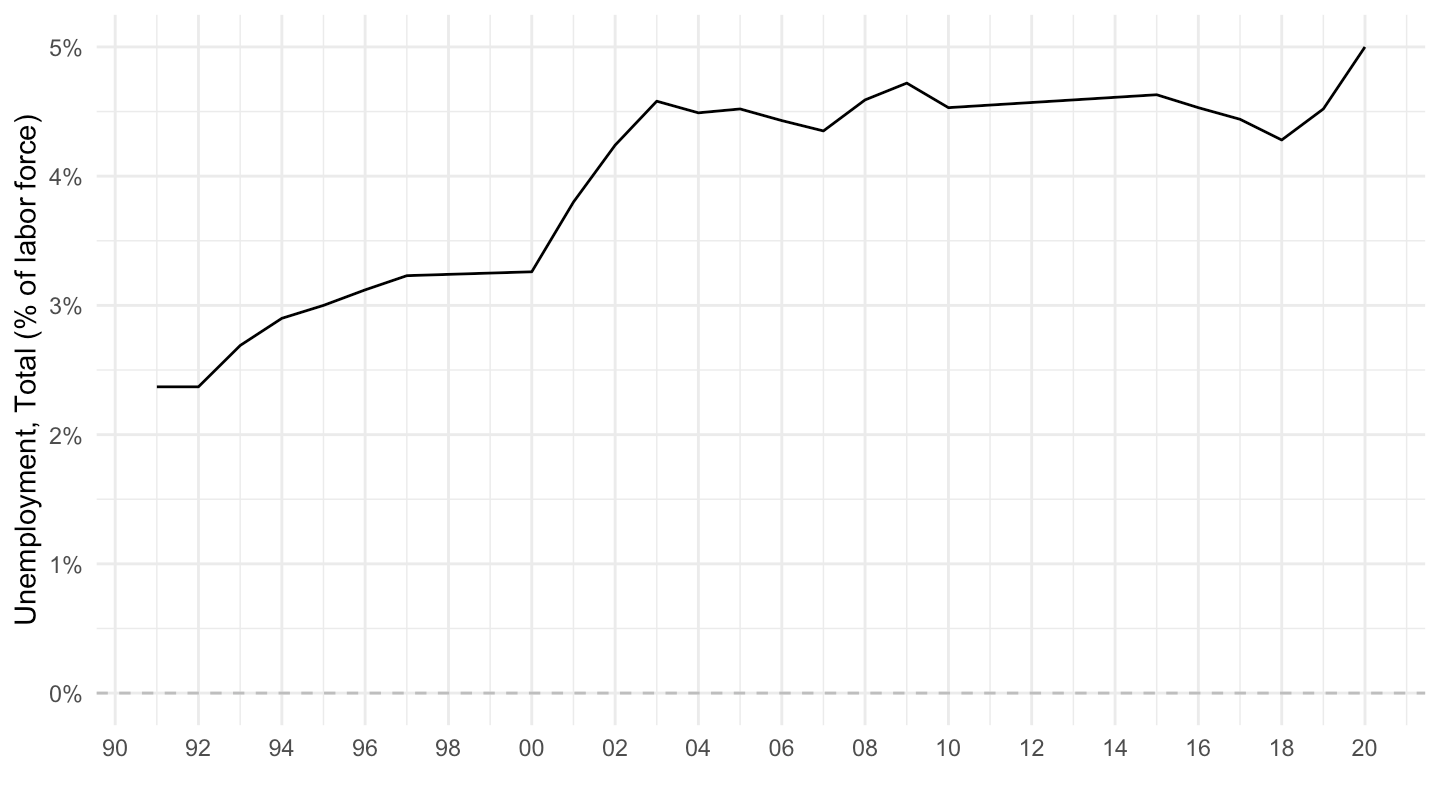
data |>
  left_join(INDICATOR) |>
  year_to_date() |>
  filter(iso2c == "VE") |>
  ggplot() + theme_minimal() + xlab("") + ylab("Unemployment (%)") +
  geom_line(aes(x = date, y = value/100, linetype = Indicator, color = Indicator)) +

  theme(legend.title = element_blank(),
        legend.position = c(0.45, 0.85)) +
  scale_x_date(breaks = seq(1900, 2100, 5) |> paste0("-01-01") |> as.Date(),
               labels = date_format("%Y")) +
  scale_y_continuous(breaks = 0.01*seq(-100, 10000, 2),
                     labels = percent_format(a = 1)) +
  geom_hline(yintercept = 0, linetype = "dashed", color = "black")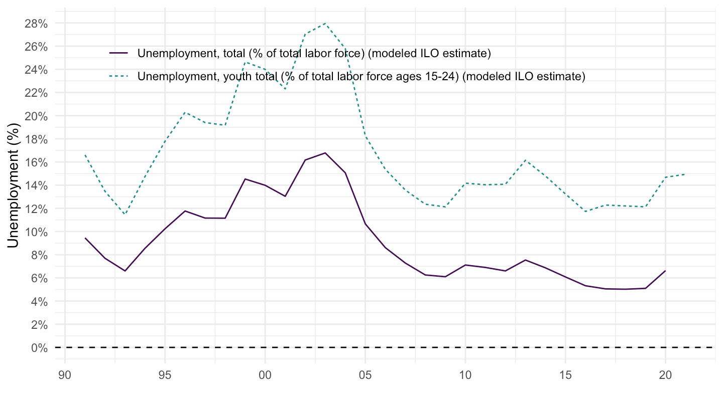
data |>
  left_join(INDICATOR) |>
  year_to_date() |>
  filter(iso2c == "FR") |>
  ggplot() + theme_minimal() + xlab("") + ylab("Unemployment (%)") +
  geom_line(aes(x = date, y = value/100, linetype = Indicator, color = Indicator)) +

  theme(legend.title = element_blank(),
        legend.position = c(0.45, 0.85)) +
  scale_x_date(breaks = seq(1900, 2100, 5) |> paste0("-01-01") |> as.Date(),
               labels = date_format("%Y")) +
  scale_y_continuous(breaks = 0.01*seq(-100, 10000, 2),
                     labels = percent_format(a = 1)) +
  geom_hline(yintercept = 0, linetype = "dashed", color = "black")