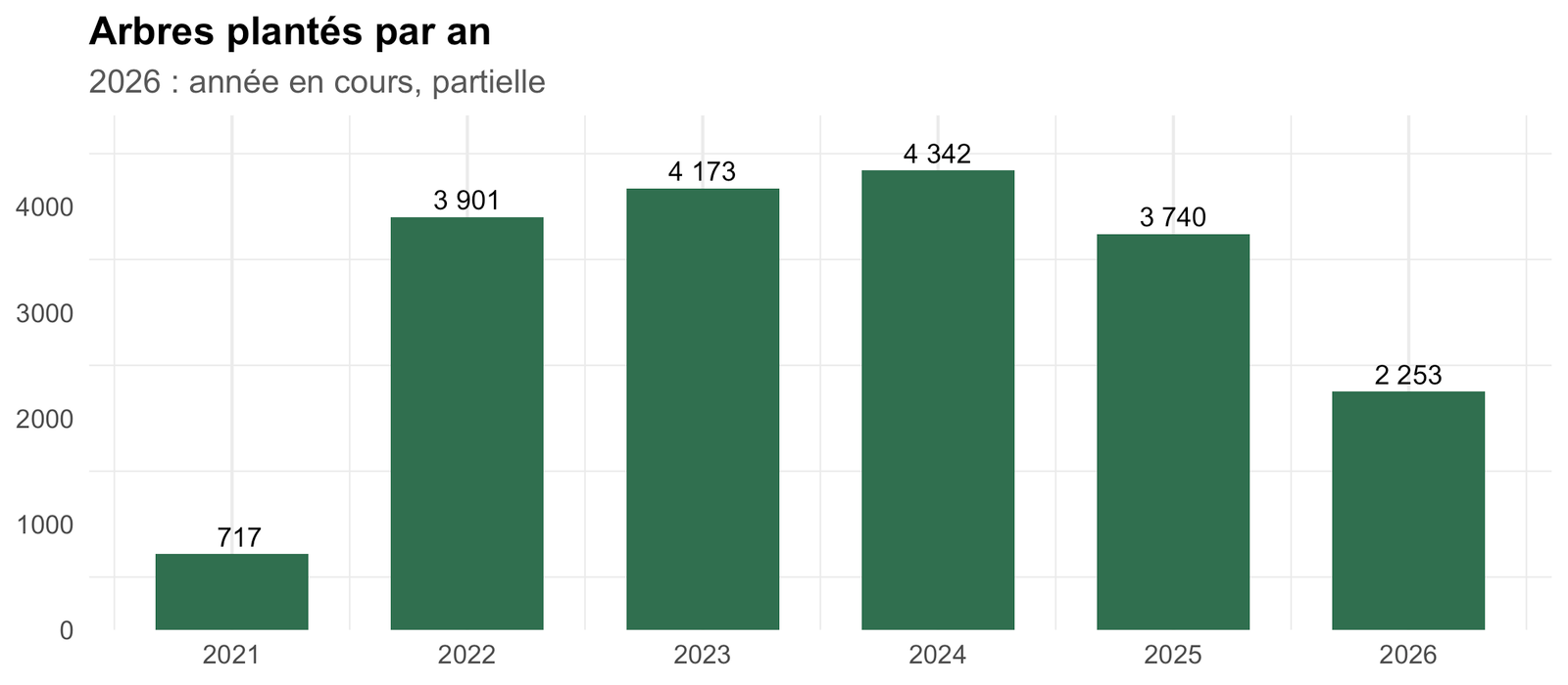
Les arbres d’alignement (plantés hors peuplement forestier)

Données - Ville de Paris

source(here::here("_rinit.R"))
source(here::here("data", "paris", "_paris.R"))   # wkb2sfc(), paris_basemap(), arrondissements_sf()
invisible(Sys.setlocale("LC_TIME", "fr_FR.UTF-8"))
invisible(Sys.setenv(TZ = "Europe/Paris"))
# cd ~/iCloud/website/data/paris; /usr/local/bin/R -e 'quarto::quarto_render("arbres-plantes-hors-peuplement-forestier.qmd")'

knitr::opts_chunk$set(echo = TRUE, message = FALSE, warning = FALSE,
                      fig.width = 8, fig.height = 5, dpi = 150)

nv_path <- here::here("data", "paris", "arbres-plantes-hors-peuplement-forestier.parquet")
nv <- arrow::read_parquet(nv_path)

xy <- sf::st_coordinates(wkb2sfc(nv$geo_point_2d))
nv <- nv |>
  dplyr::mutate(
    lon    = xy[, 1], lat = xy[, 2],
    date   = as.Date(dateplantation),
    annee  = as.integer(format(date, "%Y")),
    mois   = as.integer(format(date, "%m")),
    ar     = suppressWarnings(as.integer(stringr::str_extract(arrondissement, "[0-9]+"))),
    ar     = dplyr::if_else(stringr::str_detect(arrondissement, "PARIS"), ar, NA_integer_)
  )

n_tot     <- nrow(nv)
annee_max <- max(nv$annee)
arr_sf    <- arrondissements_sf()

theme_carte <- theme_void(base_size = 12) +
  theme(plot.title = element_text(face = "bold"),
        plot.subtitle = element_text(colour = "grey35"),
        plot.margin = margin(5, 12, 5, 5))
theme_barres <- theme_minimal(base_size = 12) +
  theme(plot.title = element_text(face = "bold"),
        plot.subtitle = element_text(colour = "grey35"),
        panel.grid.major.y = element_blank())

Les arbres plantés individuellement — hors opérations de boisement en peuplement forestier (bois de Boulogne, bois de Vincennes) — avec, pour chacun, sa date de plantation réelle. C’est le pendant « plantations récentes, arbre par arbre » du jeu arbres plantés par projet (qui, lui, raisonne par opération et dont les dates sont peu fiables) : 19 126 arbres plantés entre novembre 2021 et juin 2026.

nv |>
  dplyr::arrange(dplyr::desc(date)) |>
  dplyr::transmute(
    Date = date, Arrondissement = arrondissement, Adresse = adresse,
    `Domanialité` = domanialite, Essence = libellefrancais, Genre = genre,
    `Circonf. (cm)` = circonferenceencm, `Hauteur (m)` = hauteurenm
  ) |>
  head(10) |>
  gt::gt() |>
  gt::sub_missing(missing_text = "—") |>
  gt::tab_header(title = "10 plantations les plus récentes") |>
  gt::tab_options(table.width = "100%")

10 plantations les plus récentes
Date	Arrondissement	Adresse	Domanialité	Essence	Genre	Circonf. (cm)	Hauteur (m)
2026-06-03	PARIS 3E ARRDT	JARDINIERE DE L EGLISE DU PASSAGE SAINTE ELISABETH / 1 PASSAGE SAINTE ELISABETH	Jardin	Laurier du Portugal	Prunus	60	5
2026-06-03	PARIS 3E ARRDT	JARDINIERE DE L EGLISE DU PASSAGE SAINTE ELISABETH / 1 PASSAGE SAINTE ELISABETH	Jardin	Laurier du Portugal	Prunus	60	5
2026-06-03	PARIS 3E ARRDT	JARDINIERE DE L EGLISE DU PASSAGE SAINTE ELISABETH / 1 PASSAGE SAINTE ELISABETH	Jardin	Laurier du Portugal	Prunus	60	5
2026-05-24	PARIS 12E ARRDT	CENTRE SPORTIF ALAIN MIMOUN / 15 RUE DE LA NOUVELLE CALEDONIE	DJS	Erable	Acer	20	5
2026-05-24	PARIS 12E ARRDT	CENTRE SPORTIF ALAIN MIMOUN / 15 RUE DE LA NOUVELLE CALEDONIE	DJS	Chêne	Quercus	20	5
2026-05-18	PARIS 7E ARRDT	JARDIN DU CHAMP DE MARS ET PELOUSES DE L ECOLE MILITAIRE	Jardin	Peuplier	Populus	15	5
2026-05-18	PARIS 7E ARRDT	PROMENADE D AUSTRALIE / 14 QUAI DE BRANLY	Jardin	Charme	Carpinus	15	4
2026-05-18	PARIS 7E ARRDT	JARDIN DU CHAMP DE MARS ET PELOUSES DE L ECOLE MILITAIRE	Jardin	Hêtre	Fagus	15	5
2026-05-01	PARIS 20E ARRDT	RUE DES COURONNES	Alignement	Lilas des indes	Lagerstroemia	20	5
2026-04-29	PARIS 4E ARRDT	ECOLE POLYVALENTE / 22 RUE DE L AVE MARIA	DASCO	Parrotie de Perse	Parrotia	20	5

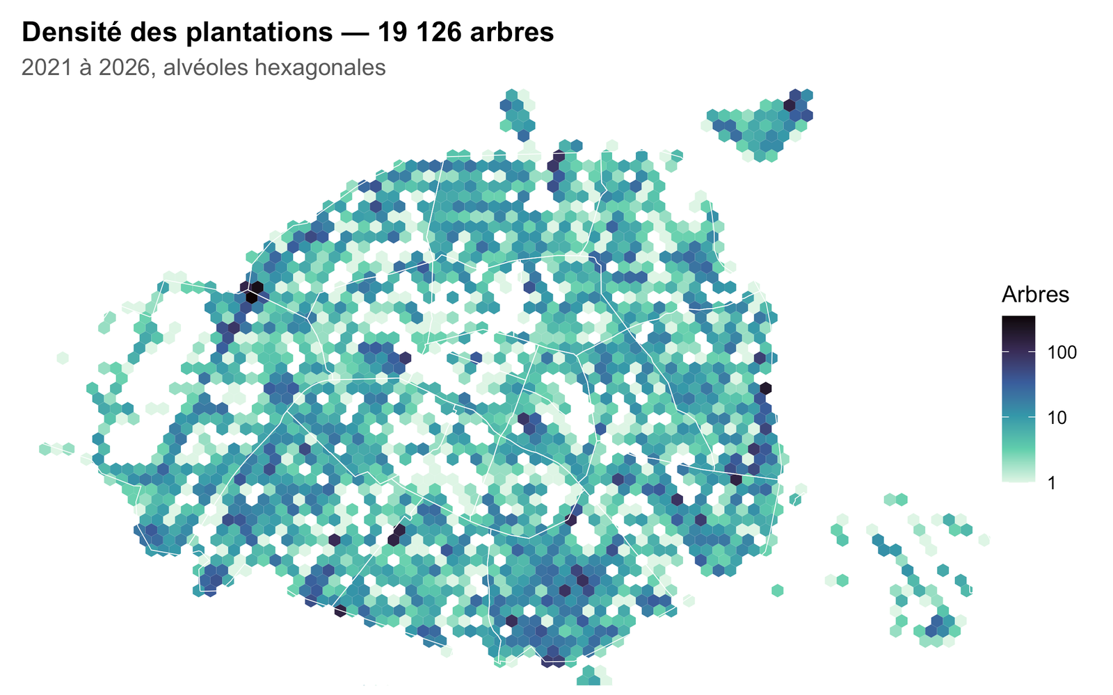
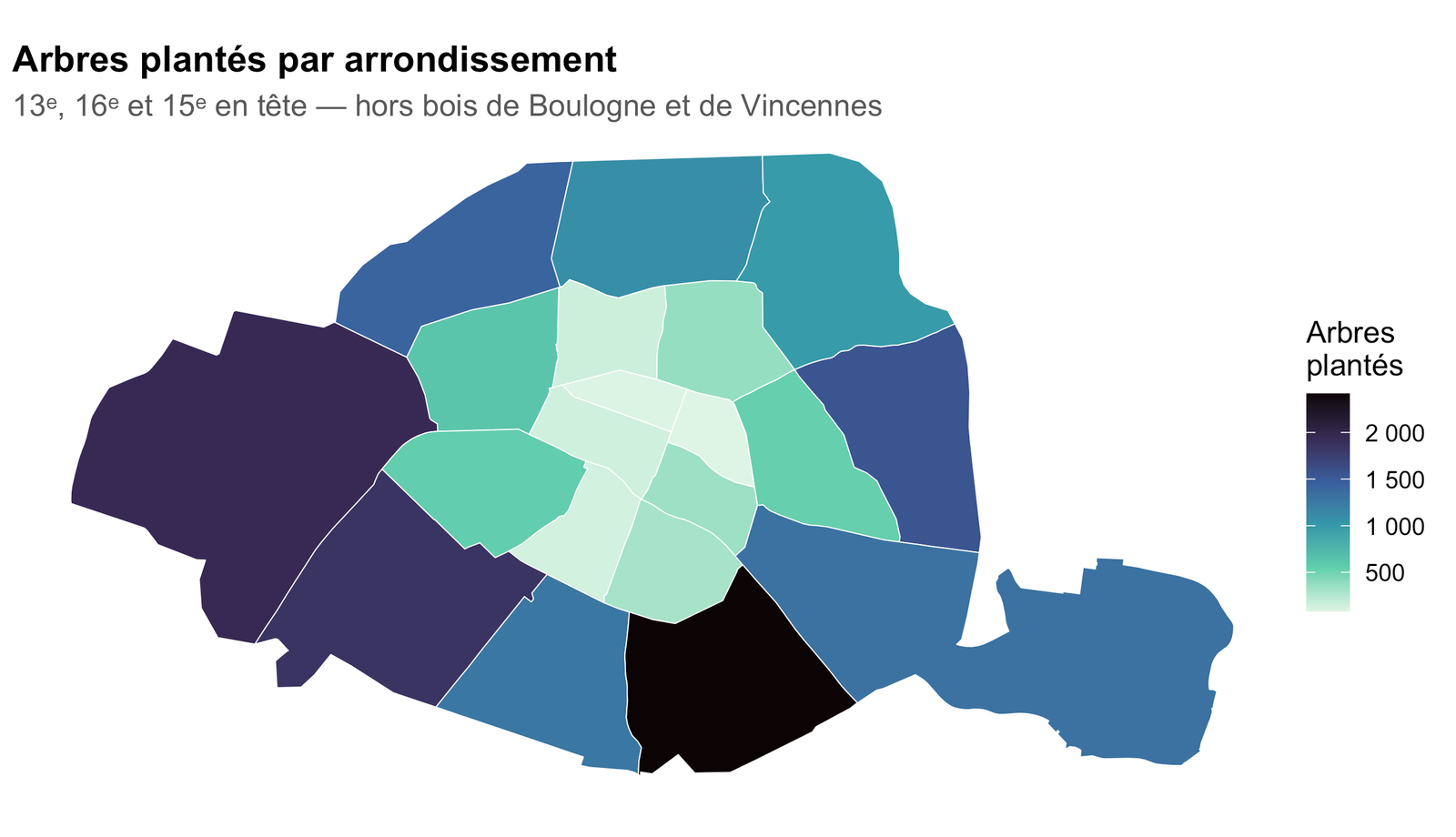
Où ont-ils été plantés

ggplot(nv, aes(lon, lat)) +
  geom_hex(bins = 80) +
  geom_sf(data = arr_sf, fill = NA, colour = "white", linewidth = 0.2, inherit.aes = FALSE) +
  scale_fill_viridis_c(option = "mako", direction = -1, trans = "log10", name = "Arbres") +
  coord_sf(xlim = c(2.222, 2.470), ylim = c(48.812, 48.914), expand = FALSE) +
  labs(title = paste0("Densité des plantations — ", format(n_tot, big.mark = " "), " arbres"),
       subtitle = "2021 à 2026, alvéoles hexagonales") +
  theme_carte

cnt <- nv |> dplyr::filter(!is.na(ar)) |> dplyr::count(ar, name = "n")

arr_sf |>
  dplyr::left_join(cnt, by = c("c_ar" = "ar")) |>
  ggplot() +
  geom_sf(aes(fill = n), colour = "white", linewidth = 0.2) +
  scale_fill_viridis_c(option = "mako", direction = -1, na.value = "grey92",
                       labels = scales::label_number(big.mark = " "), name = "Arbres\nplantés") +
  labs(title = "Arbres plantés par arrondissement",
       subtitle = "13ᵉ, 16ᵉ et 15ᵉ en tête — hors bois de Boulogne et de Vincennes") +
  theme_carte

Quand plante-t-on

nv |>
  dplyr::count(annee) |>
  dplyr::mutate(label = ifelse(annee == annee_max, paste0(annee, " (partielle)"), as.character(annee))) |>
  ggplot(aes(annee, n)) +
  geom_col(fill = "#2f6f4f", width = 0.65) +
  geom_text(aes(label = format(n, big.mark = " ")), vjust = -0.4, size = 3.5) +
  scale_x_continuous(breaks = scales::breaks_width(1)) +
  scale_y_continuous(expand = expansion(mult = c(0, 0.12))) +
  labs(title = "Arbres plantés par an",
       subtitle = paste0(annee_max, " : année en cours, partielle"),
       x = NULL, y = NULL) +
  theme_barres

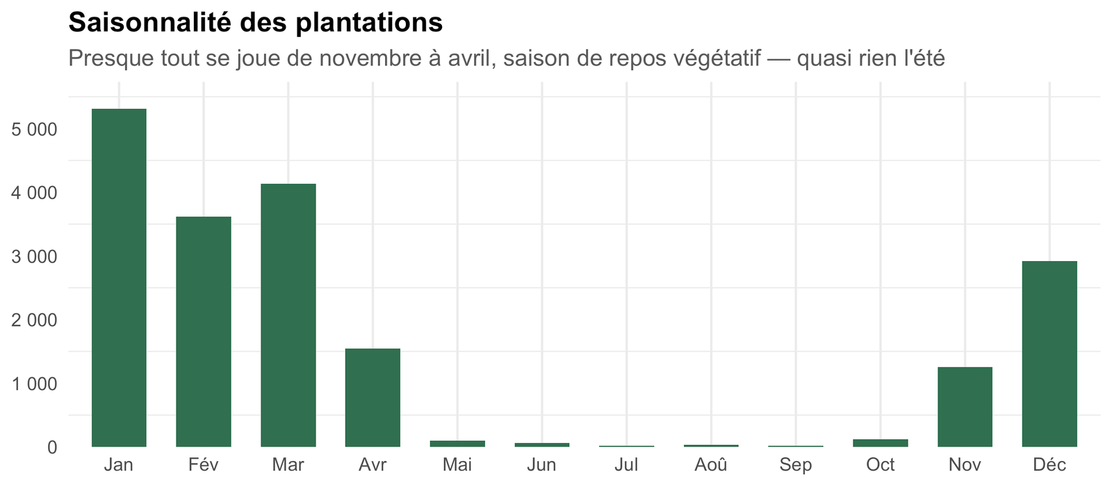
nv |>
  dplyr::count(mois) |>
  ggplot(aes(factor(mois), n)) +
  geom_col(fill = "#2f6f4f", width = 0.65) +
  scale_x_discrete(labels = c("Jan","Fév","Mar","Avr","Mai","Jun","Jul","Aoû","Sep","Oct","Nov","Déc")) +
  scale_y_continuous(labels = scales::label_number(big.mark = " "), expand = expansion(mult = c(0, 0.08))) +
  labs(title = "Saisonnalité des plantations",
       subtitle = "Presque tout se joue de novembre à avril, saison de repos végétatif — quasi rien l'été",
       x = NULL, y = NULL) +
  theme_barres

Ce que révèlent les données

Par type d’espace

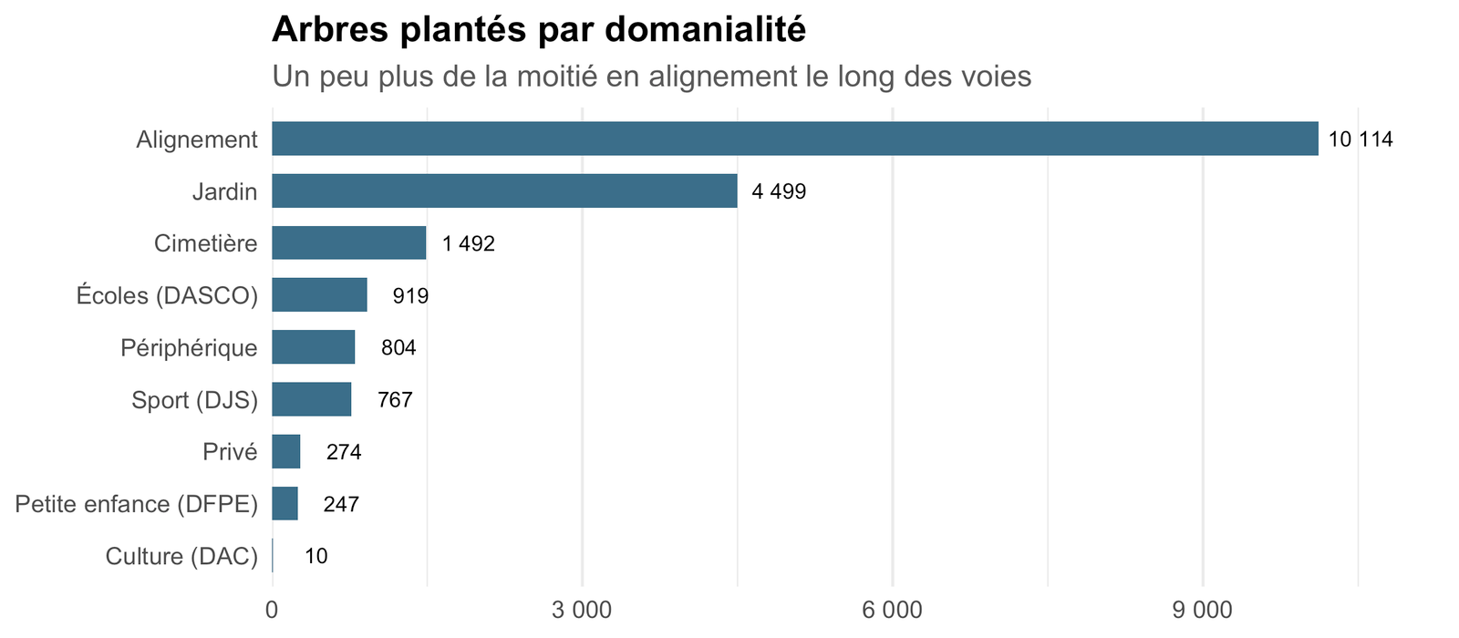
nv |>
  dplyr::mutate(domanialite = dplyr::recode(domanialite,
    DASCO = "Écoles (DASCO)", DJS = "Sport (DJS)", DFPE = "Petite enfance (DFPE)",
    DAC = "Culture (DAC)", PRIVE = "Privé")) |>
  dplyr::count(domanialite, sort = TRUE) |>
  dplyr::mutate(domanialite = forcats::fct_reorder(domanialite, n)) |>
  ggplot(aes(n, domanialite)) +
  geom_col(fill = "#3b6f8a", width = 0.65) +
  geom_text(aes(label = format(n, big.mark = " ")), hjust = -0.15, size = 3) +
  scale_x_continuous(labels = scales::label_number(big.mark = " "), expand = expansion(mult = c(0, 0.12))) +
  labs(title = "Arbres plantés par domanialité",
       subtitle = "Un peu plus de la moitié en alignement le long des voies",
       x = NULL, y = NULL) +
  theme_barres

Essences : la diversification est nette

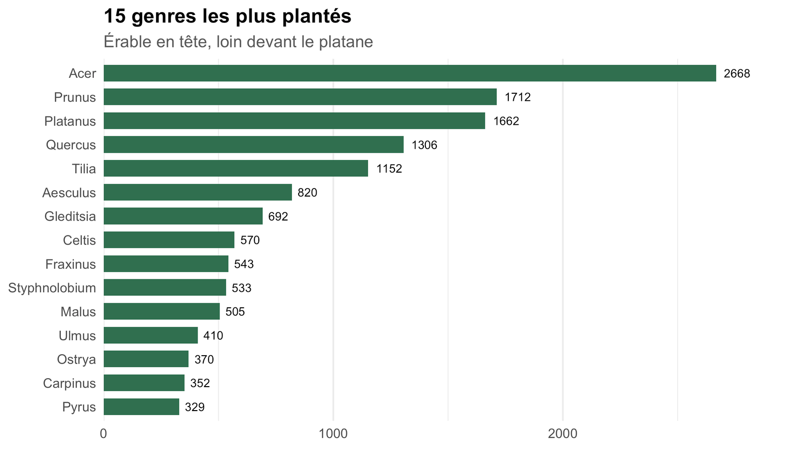
nv |>
  dplyr::filter(!is.na(genre)) |>
  dplyr::count(genre, sort = TRUE) |>
  head(15) |>
  dplyr::mutate(genre = forcats::fct_reorder(genre, n)) |>
  ggplot(aes(n, genre)) +
  geom_col(fill = "#2f6f4f", width = 0.7) +
  geom_text(aes(label = n), hjust = -0.3, size = 3) +
  scale_x_continuous(expand = expansion(mult = c(0, 0.12))) +
  labs(title = "15 genres les plus plantés",
       subtitle = "Érable en tête, loin devant le platane",
       x = NULL, y = NULL) +
  theme_barres

la_path <- here::here("data", "paris", "les-arbres.parquet")
if (file.exists(la_path)) {
  la <- arrow::read_parquet(la_path, col_select = "genre")
  part_new <- mean(nv$genre == "Platanus", na.rm = TRUE)
  part_old <- mean(la$genre == "Platanus", na.rm = TRUE)
  cat(sprintf(
    "\nLe platane pesait **%s** du [patrimoine arboré existant](les-arbres.html) ; il ne représente plus que **%s** des arbres plantés depuis 2021 — la Ville diversifie nettement ses plantations (moindre vulnérabilité aux maladies, résilience climatique).\n",
    scales::percent(part_old, 0.1), scales::percent(part_new, 0.1)))
}

Le platane pesait 19.5% du patrimoine arboré existant ; il ne représente plus que 8.7% des arbres plantés depuis 2021 — la Ville diversifie nettement ses plantations (moindre vulnérabilité aux maladies, résilience climatique).

Source & données

tibble::tibble(
  ` ` = c("Jeu de données", "Producteur", "Licence", "Fichiers", "Mise à jour", "Observations"),
  `  ` = c(
    "[Les arbres d'alignement (plantés hors peuplement forestier)](https://opendata.paris.fr/explore/dataset/arbres-plantes-hors-peuplement-forestier/information/)",
    "Direction des Espaces Verts et de l'Environnement (DEVE) — Ville de Paris",
    "Open Database License (ODbL)",
    sprintf("`data/paris/arbres-plantes-hors-peuplement-forestier.parquet` (%s ko) + `arrondissements.parquet`",
            round(file.size(nv_path) / 1024)),
    format(as.Date(file.mtime(nv_path)), "%d %B %Y"),
    sprintf("%s arbres, plantés entre %s et %s", format(n_tot, big.mark = " "),
            format(min(nv$date), "%Y-%m"), format(max(nv$date), "%Y-%m"))
  )
) |>
  gt::gt() |> gt::fmt_markdown(columns = `  `) |>
  gt::tab_options(table.width = "100%", column_labels.hidden = TRUE)

Jeu de données	Les arbres d’alignement (plantés hors peuplement forestier)
Producteur	Direction des Espaces Verts et de l’Environnement (DEVE) — Ville de Paris
Licence	Open Database License (ODbL)
Fichiers	data/paris/arbres-plantes-hors-peuplement-forestier.parquet (876 ko) + arrondissements.parquet
Mise à jour	04 septembre 2026
Observations	19 126 arbres, plantés entre 2021-11 et 2026-06

• Les arbres de Paris — inventaire
• Arbres plantés par la Ville de Paris, par projet
• Arbres abattus pour raisons sanitaires et essence de remplacement
• Les arbres remarquables de Paris
• Catalogue des données ouvertes de la Ville de Paris · Jeux de données traités ici