| source | dataset | .html | .RData |
|---|---|---|---|
| oecd | QNA | 2024-05-05 | 2024-04-15 |
Quarterly National Accounts
Data - OECD
Info
Last
| obsTime | Nobs |
|---|---|
| 2024-Q1 | 1804 |
TRANSACTION
Code
QNA %>%
  left_join(TRANSACTION, by = "TRANSACTION") %>%
  group_by(TRANSACTION, Transaction) %>%
  summarise(Nobs = n()) %>%
  arrange(-Nobs) %>%
  print_table_conditional()
ACTIVITY
Code
QNA %>%
  left_join(ACTIVITY, by = "ACTIVITY") %>%
  group_by(ACTIVITY, Activity) %>%
  summarise(Nobs = n()) %>%
  arrange(-Nobs) %>%
print_table_conditional()| ACTIVITY | Activity | Nobs |
|---|---|---|
| _Z | Not applicable | 1575834 |
| _T | Total - All activities | 646402 |
| A | Agriculture, forestry and fishing | 114505 |
| F | Construction | 114001 |
| C | Manufacturing | 113292 |
| BTE | Industry (except construction) | 113069 |
| J | Information and communication | 112994 |
| K | Financial and insurance activities | 112833 |
| GTI | Wholesale and retail trade; repair of motor vehicles and motorcycles; transportation and storage; accommodation and food service activities | 112455 |
| L | Real estate activities | 112364 |
| OTQ | Public administration, defence, education, human health and social work activities | 112331 |
| RTU | Arts, entertainment and recreation; other service activities; activities of household and extra-territorial organizations and bodies | 112234 |
| M_N | Professional, scientific and technical activities; administrative and support service activities | 111465 |
| GTU | Services | 24842 |
SECTOR
Code
QNA %>%
  left_join(SECTOR, by = "SECTOR") %>%
  group_by(SECTOR, Sector) %>%
  summarise(Nobs = n()) %>%
  arrange(-Nobs) %>%
print_table_conditional()| SECTOR | Sector | Nobs |
|---|---|---|
| S1 | Total economy | 2961165 |
| S13 | General government | 192698 |
| S14 | Households | 156710 |
| S1M | Households and non-profit institutions serving households (NPISH) | 144107 |
| S15 | Non-profit institutions serving households | 25727 |
| S1W | Other sectors than general government | 8214 |
PRICE_BASE
Code
QNA %>%
  left_join(PRICE_BASE, by = "PRICE_BASE") %>%
  group_by(PRICE_BASE, Price_base) %>%
  summarise(Nobs = n()) %>%
  arrange(-Nobs) %>%
print_table_conditional()| PRICE_BASE | Price_base | Nobs |
|---|---|---|
| V | Current prices | 1471066 |
| L | Chain linked volume | 861148 |
| _Z | Not applicable | 749553 |
| LR | Chain linked volume (rebased) | 225675 |
| DR | Deflator (rebased) | 64404 |
| D | Deflator | 60350 |
| Q | Constant prices | 44621 |
| QR | Constant prices (rebased) | 11804 |
REF_AREA
Code
QNA %>%
  left_join(REF_AREA, by = "REF_AREA") %>%
  group_by(REF_AREA, Ref_area) %>%
  summarise(Nobs = n()) %>%
  arrange(-Nobs) %>%
  print_table_conditional()
TABLE_IDENTIFIER
Code
QNA %>%
  left_join(TABLE_IDENTIFIER, by = "TABLE_IDENTIFIER") %>%
  group_by(TABLE_IDENTIFIER, Table_identifier) %>%
  summarise(Nobs = n()) %>%
  arrange(-Nobs) %>%
print_table_conditional()| TABLE_IDENTIFIER | Table_identifier | Nobs |
|---|---|---|
| T0102 | Table 0102 - GDP identity from the expenditure side | 1597574 |
| T0111 | Table 0111 - Employment by industry | 705258 |
| T0101 | Table 0101 - Gross value added at basic prices and gross domestic product at market prices | 440439 |
| T0103 | Table 0103 - GDP identity from the income side | 405337 |
| T0107 | Table 0107 - Disposable income, saving, net lending / borrowing | 164892 |
| T0117 | Table 0117 - Final consumption expenditure of households by durability | 130826 |
| T0110 | Table 0110 - Population and employment | 44295 |
UNIT_MEASURE
Code
QNA %>%
  left_join(UNIT_MEASURE, by = "UNIT_MEASURE") %>%
  group_by(UNIT_MEASURE, Unit_measure) %>%
  summarise(Nobs = n()) %>%
  arrange(-Nobs) %>%
print_table_conditional()| UNIT_MEASURE | Unit_measure | Nobs |
|---|---|---|
| XDC | National currency | 2173615 |
| PS | Persons | 398522 |
| H | Hours | 335731 |
| IX | Index | 188068 |
| USD_PPP | US dollars, PPP converted | 166280 |
| PC | Percentage change | 166242 |
| PD | Percentage points | 18095 |
| JB | Jobs | 15300 |
| USD_PPP_PS | US dollars per person, PPP converted | 14489 |
| XDC_USD | National currency per US dollar | 12279 |
TRANSFORMATION
Code
QNA %>%
  left_join(TRANSFORMATION, by = "TRANSFORMATION") %>%
  group_by(TRANSFORMATION, Transformation) %>%
  summarise(Nobs = n()) %>%
  arrange(-Nobs) %>%
print_table_conditional()| TRANSFORMATION | Transformation | Nobs |
|---|---|---|
| N | Non transformed data | 2852736 |
| LA | Annual levels | 451548 |
| G1 | Growth rate, period on period | 81016 |
| GY | Growth rate, over 1 year | 80074 |
| GO1 | Contribution to growth rate, period on period | 18095 |
| GCM | Cumulative growth rate since base period | 5152 |
U.S., Europe
B1GQ_POP
1995-
Code
QNA %>%
  filter(REF_AREA %in% c("USA", "EA20"),
         FREQ == "Q",
         TRANSACTION == "B1GQ_POP",
         PRICE_BASE == "LR") %>%
  quarter_to_date %>%
  filter(date >= as.Date("1995-01-01")) %>%
  mutate(Location = ifelse(REF_AREA == "USA", "United States", "Europe")) %>%
  group_by(Location) %>%
  arrange(date) %>%
  mutate(obsValue = 100 * obsValue / obsValue[1]) %>%
  left_join(colors, by = c("Location" = "country")) %>%
  mutate(color = ifelse(REF_AREA == "USA", color2, color)) %>%
  ggplot(.) + theme_minimal() + xlab("") + ylab("PIB par habitant (1995 = 100)") +
  geom_line(aes(x = date, y = obsValue, color = color)) + add_2flags +
  scale_color_identity() +
  scale_x_date(breaks = seq(1960, 2100, 2) %>% paste0("-01-01") %>% as.Date,
               labels = date_format("%Y")) +
  theme(legend.position = "none") +
  scale_y_log10(breaks = seq(50, 200, 5))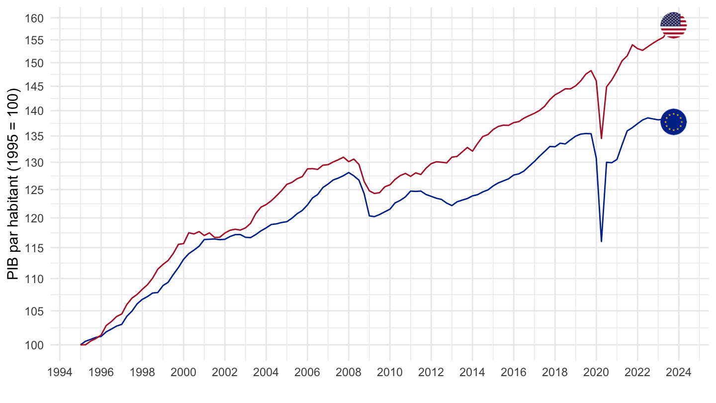
1999-
Code
plot <- QNA %>%
  filter(REF_AREA %in% c("USA", "EA20"),
         FREQ == "Q",
         TRANSACTION == "B1GQ_POP",
         PRICE_BASE == "LR") %>%
  quarter_to_date %>%
  filter(date >= as.Date("1999-01-01")) %>%
  mutate(Location = ifelse(REF_AREA == "USA", "United States", "Europe")) %>%
  group_by(Location) %>%
  arrange(date) %>%
  mutate(obsValue = 100 * obsValue / obsValue[1]) %>%
  left_join(colors, by = c("Location" = "country")) %>%
  mutate(color = ifelse(REF_AREA == "USA", color2, color)) %>%
  ggplot(.) + theme_minimal() + xlab("") + ylab("PIB par habitant (1999T1 = 100)") +
  geom_line(aes(x = date, y = obsValue, color = color)) + add_2flags +
  scale_color_identity() +
  scale_x_date(breaks = c(seq(1999, 2100, 5), seq(1997, 2100, 5)) %>% paste0("-01-01") %>% as.Date,
               labels = date_format("%Y")) +
  theme(legend.position = "none") +
  scale_y_log10(breaks = seq(50, 200, 5))

plot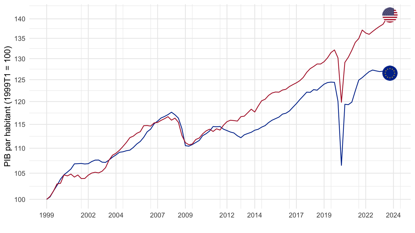
Code
save(plot, file = "QNA_files/figure-html/USA-EA20-1999-1.RData")2000-
Code
QNA %>%
  filter(REF_AREA %in% c("USA", "EA20"),
         FREQ == "Q",
         TRANSACTION == "B1GQ_POP",
         PRICE_BASE == "LR")  %>%
  quarter_to_date %>%
  filter(date >= as.Date("2000-01-01")) %>%
  mutate(Location = ifelse(REF_AREA == "USA", "United States", "Europe")) %>%
  group_by(Location) %>%
  arrange(date) %>%
  mutate(obsValue = 100 * obsValue / obsValue[1]) %>%
  left_join(colors, by = c("Location" = "country")) %>%
  mutate(color = ifelse(REF_AREA == "USA", color2, color)) %>%
  ggplot(.) + theme_minimal() + xlab("") + ylab("PIB par habitant (2000 = 100)") +
  geom_line(aes(x = date, y = obsValue, color = color)) + add_2flags +
  scale_color_identity() +
  scale_x_date(breaks = seq(1960, 2100, 2) %>% paste0("-01-01") %>% as.Date,
               labels = date_format("%Y")) +
  theme(legend.position = "none") +
  scale_y_log10(breaks = seq(50, 200, 5))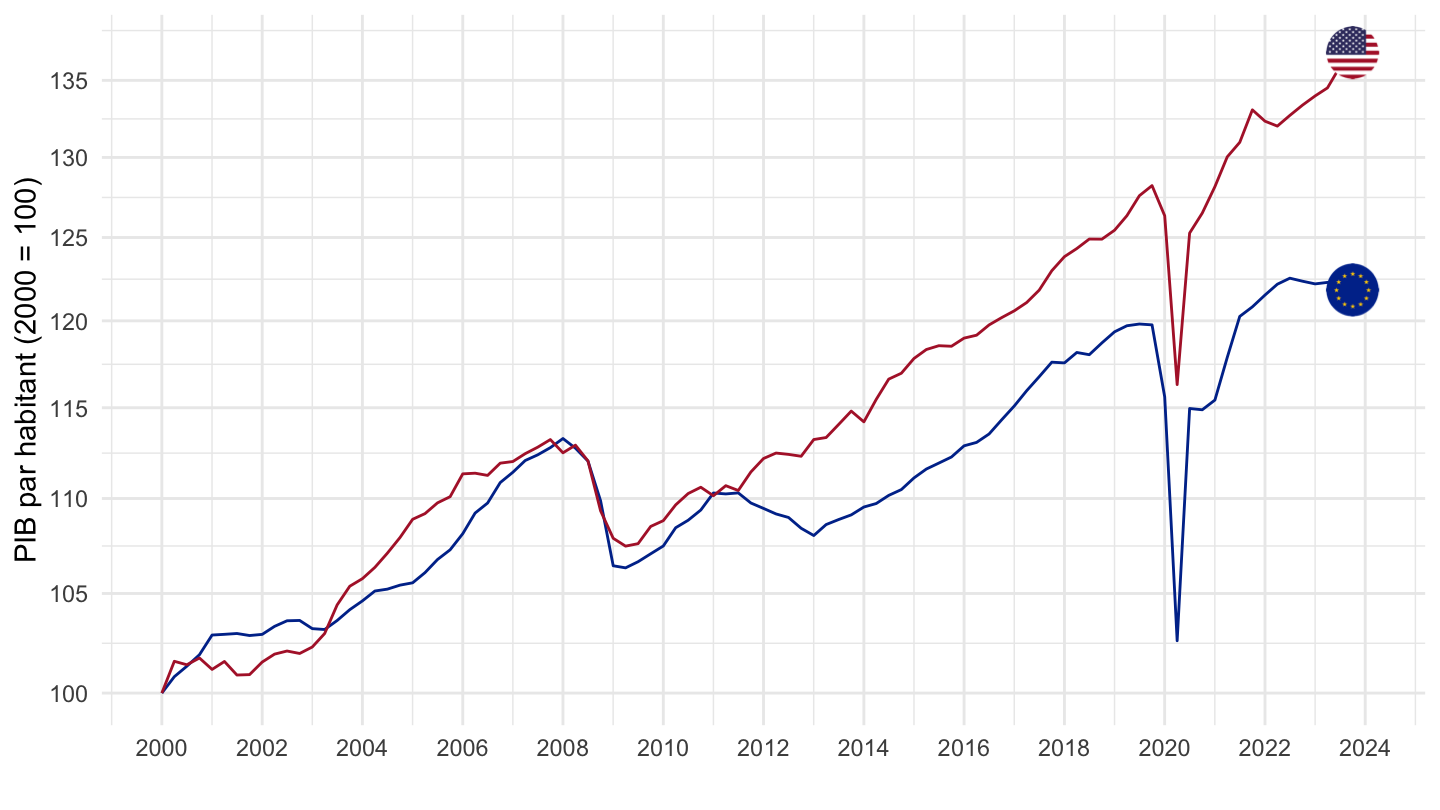
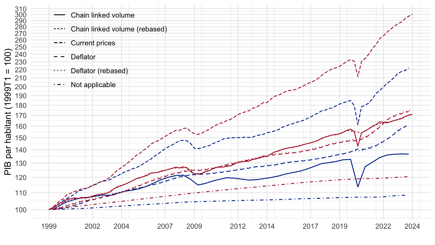
B1GQ
1999-
Absolute
Code
QNA %>%
  filter(REF_AREA %in% c("USA", "EA20"),
         FREQ == "Q",
         TRANSACTION == "B1GQ",
         TRANSFORMATION == "N",
         ADJUSTMENT == "Y") %>%
  quarter_to_date %>%
  filter(date >= as.Date("1999-01-01")) %>%
  arrange(desc(date)) %>%
  mutate(Location = ifelse(REF_AREA == "USA", "United States", "Europe")) %>%
  group_by(Location, PRICE_BASE) %>%
  arrange(date) %>%
  mutate(obsValue = 100 * obsValue / obsValue[1]) %>%
  left_join(colors, by = c("Location" = "country")) %>%
  mutate(color = ifelse(REF_AREA == "USA", color2, color)) %>%
  left_join(PRICE_BASE, by = "PRICE_BASE") %>%
  ggplot(.) + theme_minimal() + xlab("") + ylab("PIB par habitant (1999T1 = 100)") +
  geom_line(aes(x = date, y = obsValue, color = color, linetype = Price_base)) + add_2flags +
  scale_color_identity() +
  scale_x_date(breaks = c(seq(1999, 2100, 5), seq(1997, 2100, 5)) %>% paste0("-01-01") %>% as.Date,
               labels = date_format("%Y")) +
  theme(legend.position = c(0.2, 0.8),
        legend.title = element_blank()) +
  scale_y_log10(breaks = seq(50, 500, 10))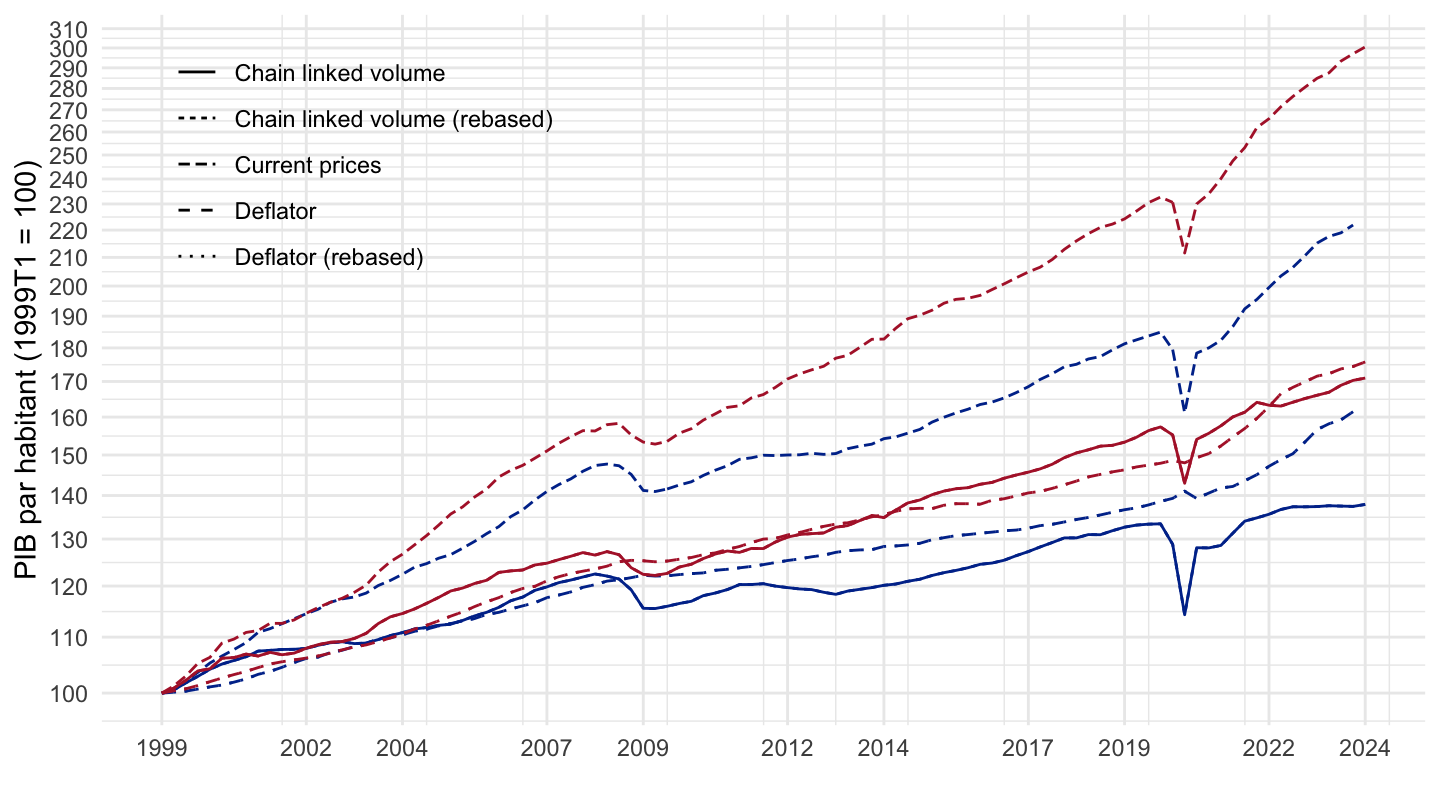
Per capita
Code
QNA %>%
  filter(REF_AREA %in% c("USA", "EA20"),
         FREQ == "Q",
         TRANSACTION == c("B1GQ", "POP"),
         TRANSFORMATION == "N",
         ADJUSTMENT == "Y") %>%
  quarter_to_date %>%
  filter(date >= as.Date("1999-01-01")) %>%
  arrange(desc(date)) %>%
  mutate(Location = ifelse(REF_AREA == "USA", "United States", "Europe")) %>%
  group_by(Location, PRICE_BASE) %>%
  arrange(date) %>%
  mutate(obsValue = 100 * obsValue / obsValue[1]) %>%
  left_join(colors, by = c("Location" = "country")) %>%
  mutate(color = ifelse(REF_AREA == "USA", color2, color)) %>%
  left_join(PRICE_BASE, by = "PRICE_BASE") %>%
  ggplot(.) + theme_minimal() + xlab("") + ylab("PIB par habitant (1999T1 = 100)") +
  geom_line(aes(x = date, y = obsValue, color = color, linetype = Price_base)) + add_2flags +
  scale_color_identity() +
  scale_x_date(breaks = c(seq(1999, 2100, 5), seq(1997, 2100, 5)) %>% paste0("-01-01") %>% as.Date,
               labels = date_format("%Y")) +
  theme(legend.position = c(0.2, 0.8),
        legend.title = element_blank()) +
  scale_y_log10(breaks = seq(50, 500, 10))