Last observation: Q4 2025 (N = 1) · 2025 (N = 1)
First observation: 1960 (N = 1627) · Q1 1960 (N = 1146)
Last data update: 02 août 2026, 08:59
Last compile: 09 oct. 2026, 23:08
EO110_INTERNET |>
  mutate(vintage = "Economic Outlook No 110 - December 2021") |>
  bind_rows(EO111_INTERNET |>
              mutate(vintage = "Economic Outlook No 111 - June 2022")) |>
  bind_rows(EO112_INTERNET |>
              mutate(vintage = "Economic Outlook No 112 - November 2022")) |>
  bind_rows(EO113_INTERNET |>
              mutate(vintage = "Economic Outlook No 113 - June 2023")) |>
  filter(VARIABLE == "GDPV",
         LOCATION == "LTU",
         FREQUENCY == "Q") |>
  quarter_to_date() |>
  filter(date >= as.Date("2021-01-01")) |>
  group_by(vintage) |>
  mutate(obsValue = 100*obsValue/obsValue[date == as.Date("2021-01-01")]) |>
  ggplot() + geom_line(aes(x = date, y = obsValue, color = vintage)) +
  xlab("") + ylab("Gross Domestic Product in Volume, Lithuania") + theme_minimal() +
  scale_x_date(breaks = seq(1920, 2100, 1) |> paste0("-01-01") |> as.Date(),
               labels = date_format("%Y")) +
  theme(legend.position = c(0.7, 0.2),
        legend.title = element_blank()) +
  scale_y_log10(breaks = seq(20, 200, 1))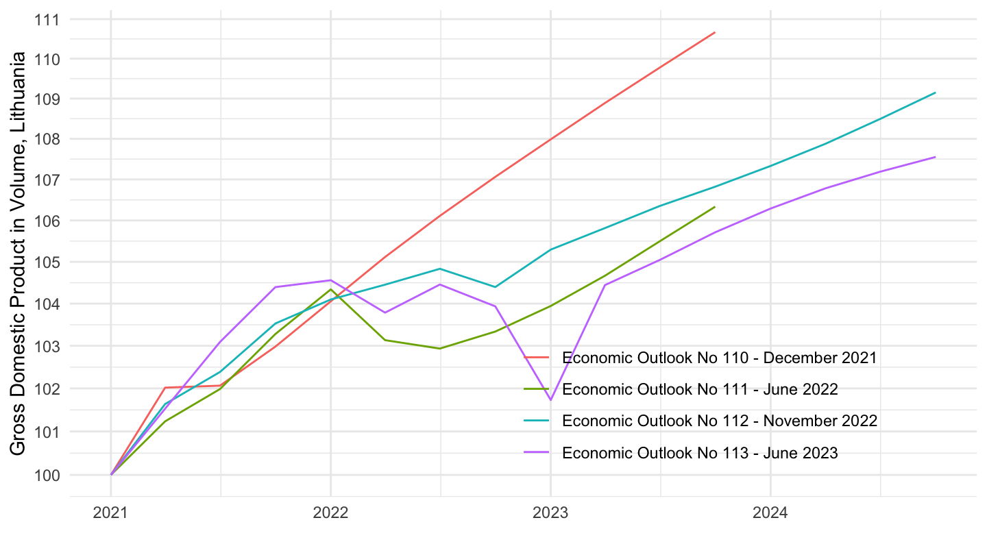
EO110_INTERNET |>
  mutate(vintage = "Economic Outlook No 110 - December 2021") |>
  bind_rows(EO111_INTERNET |>
              mutate(vintage = "Economic Outlook No 111 - June 2022")) |>
  bind_rows(EO112_INTERNET |>
              mutate(vintage = "Economic Outlook No 112 - November 2022")) |>
  bind_rows(EO113_INTERNET |>
              mutate(vintage = "Economic Outlook No 113 - June 2023")) |>
  filter(VARIABLE == "GDPV",
         LOCATION == "SVK",
         FREQUENCY == "Q") |>
  quarter_to_date() |>
  filter(date >= as.Date("2021-01-01")) |>
  group_by(vintage) |>
  mutate(obsValue = 100*obsValue/obsValue[date == as.Date("2021-01-01")]) |>
  ggplot() + geom_line(aes(x = date, y = obsValue, color = vintage)) +
  xlab("") + ylab("Gross Domestic Product in Volume, Slovakia") + theme_minimal() +
  scale_x_date(breaks = seq(1920, 2100, 1) |> paste0("-01-01") |> as.Date(),
               labels = date_format("%Y")) +
  theme(legend.position = c(0.7, 0.2),
        legend.title = element_blank()) +
  scale_y_log10(breaks = seq(20, 200, 1))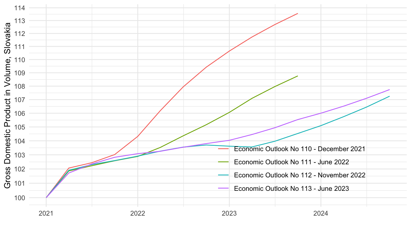
EO110_INTERNET |>
  mutate(vintage = "Economic Outlook No 110 - December 2021") |>
  bind_rows(EO111_INTERNET |>
              mutate(vintage = "Economic Outlook No 111 - June 2022")) |>
  bind_rows(EO112_INTERNET |>
              mutate(vintage = "Economic Outlook No 112 - November 2022")) |>
  bind_rows(EO113_INTERNET |>
              mutate(vintage = "Economic Outlook No 113 - June 2023")) |>
  filter(VARIABLE == "GDPV",
         LOCATION == "FIN",
         FREQUENCY == "Q") |>
  quarter_to_date() |>
  filter(date >= as.Date("2021-01-01")) |>
  group_by(vintage) |>
  mutate(obsValue = 100*obsValue/obsValue[date == as.Date("2021-01-01")]) |>
  ggplot() + geom_line(aes(x = date, y = obsValue, color = vintage)) +
  xlab("") + ylab("Gross Domestic Product in Volume, Finland") + theme_minimal() +
  scale_x_date(breaks = seq(1920, 2100, 1) |> paste0("-01-01") |> as.Date(),
               labels = date_format("%Y")) +
  theme(legend.position = c(0.7, 0.2),
        legend.title = element_blank()) +
  scale_y_log10(breaks = seq(20, 200, 1))
EO113_INTERNET |>
              mutate(vintage = "EO No 113 - June 2023") |>
  bind_rows(EO110_INTERNET |>
              mutate(vintage = "EO No 110 - December 2021")) |>
  filter(LOCATION == "DEU",
         obsTime == "2023-Q1",
         VARIABLE %in% c("GDPV", "ITV", "CPV", "CGV", "MGSV", "XGSV"),
         FREQUENCY == "Q") |>
  left_join(EO113_INTERNET_var$VARIABLE, by = "VARIABLE") |>
  select(VARIABLE, Variable, UNIT, vintage, obsValue) |>
  spread(vintage, obsValue) |>
  mutate(`Change (%)` = round(100*(`EO No 113 - June 2023`/`EO No 110 - December 2021`-1), 2)) |>
print_table_conditional()| VARIABLE | Variable | UNIT | EO No 110 - December 2021 | EO No 113 - June 2023 | Change (%) |
|---|---|---|---|---|---|
| CGV | Government final consumption expenditure, volume | EUR | 7.079714e+11 | 6.749840e+11 | -4.66 |
| CPV | Private final consumption expenditure, volume | EUR | 1.764611e+12 | 1.673660e+12 | -5.15 |
| GDPV | Gross domestic product, volume, market prices | EUR | 3.360288e+12 | 3.238844e+12 | -3.61 |
| ITV | Gross fixed capital formation, total, volume | EUR | 7.141888e+11 | 6.806400e+11 | -4.70 |
| MGSV | Imports of goods and services, volume (national accounts basis) | EUR | 1.476323e+12 | 1.472700e+12 | -0.25 |
| XGSV | Exports of goods and services, volume (national accounts basis) | EUR | 1.634885e+12 | 1.623416e+12 | -0.70 |
EO113_INTERNET |>
              mutate(vintage = "EO No 113 - June 2023") |>
  bind_rows(EO110_INTERNET |>
              mutate(vintage = "EO No 110 - December 2021")) |>
  filter(LOCATION == "DEU",
         obsTime == "2023-Q1",
         FREQUENCY == "Q") |>
  left_join(EO113_INTERNET_var$VARIABLE, by = "VARIABLE") |>
  select(VARIABLE, Variable, UNIT, vintage, obsValue) |>
  spread(vintage, obsValue) |>
  mutate(`Change (%)` = round(100*(`EO No 113 - June 2023`/`EO No 110 - December 2021`-1), 2)) |>
print_table_conditional()EO110_INTERNET |>
mutate(vintage = "Economic Outlook No 110 - December 2021") |>
bind_rows(EO111_INTERNET |>
mutate(vintage = "Economic Outlook No 111 - June 2022")) |>
bind_rows(EO112_INTERNET |>
mutate(vintage = "Economic Outlook No 112 - November 2022")) |>
bind_rows(EO113_INTERNET |>
mutate(vintage = "Economic Outlook No 113 - June 2023")) |>
filter(VARIABLE == "GDPV",
LOCATION == "DEU",
FREQUENCY == "Q") |>
quarter_to_date() |>
filter(date >= as.Date("2014-01-01")) |>
group_by(vintage) |>
mutate(obsValue = 100*obsValue/obsValue[date == as.Date("2014-01-01")]) |>
ggplot() + geom_line(aes(x = date, y = obsValue, color = vintage)) +
xlab("") + ylab("Gross Domestic Product in Volume, Germany") + theme_minimal() +
scale_x_date(breaks = seq(1920, 2100, 1) |> paste0("-01-01") |> as.Date(),
labels = date_format("%Y")) +
theme(legend.position = c(0.25, 0.9),
legend.title = element_blank()) +
scale_y_log10(breaks = seq(20, 200, 1))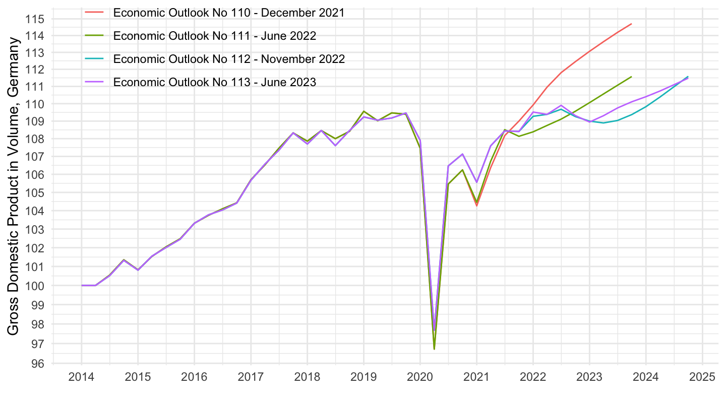
EO110_INTERNET |>
  mutate(vintage = "Economic Outlook No 110 - December 2021") |>
  bind_rows(EO111_INTERNET |>
              mutate(vintage = "Economic Outlook No 111 - June 2022")) |>
  bind_rows(EO112_INTERNET |>
              mutate(vintage = "Economic Outlook No 112 - November 2022")) |>
  bind_rows(EO113_INTERNET |>
              mutate(vintage = "Economic Outlook No 113 - June 2023")) |>
  filter(VARIABLE == "GDPV",
         LOCATION == "DEU",
         FREQUENCY == "Q") |>
  quarter_to_date() |>
  filter(date >= as.Date("2017-01-01")) |>
  group_by(vintage) |>
  mutate(obsValue = 100*obsValue/obsValue[date == as.Date("2017-01-01")]) |>
  ggplot() + geom_line(aes(x = date, y = obsValue, color = vintage)) +
  xlab("") + ylab("Gross Domestic Product in Volume, Germany") + theme_minimal() +
  scale_x_date(breaks = seq(1920, 2100, 1) |> paste0("-01-01") |> as.Date(),
               labels = date_format("%Y")) +
  theme(legend.position = c(0.7, 0.2),
        legend.title = element_blank()) +
  scale_y_log10(breaks = seq(20, 200, 1))
EO110_INTERNET |>
  mutate(vintage = "Economic Outlook No 110 - December 2021") |>
  bind_rows(EO111_INTERNET |>
              mutate(vintage = "Economic Outlook No 111 - June 2022")) |>
  bind_rows(EO112_INTERNET |>
              mutate(vintage = "Economic Outlook No 112 - November 2022")) |>
  bind_rows(EO113_INTERNET |>
              mutate(vintage = "Economic Outlook No 113 - June 2023")) |>
  filter(VARIABLE == "GDPV",
         LOCATION == "DEU",
         FREQUENCY == "Q") |>
  quarter_to_date() |>
  filter(date >= as.Date("2021-01-01")) |>
  group_by(vintage) |>
  mutate(obsValue = 100*obsValue/obsValue[date == as.Date("2021-01-01")]) |>
  ggplot() + geom_line(aes(x = date, y = obsValue, color = vintage)) +
  xlab("") + ylab("Gross Domestic Product in Volume, Germany") + theme_minimal() +
  scale_x_date(breaks = seq(1920, 2100, 1) |> paste0("-01-01") |> as.Date(),
               labels = date_format("%Y")) +
  theme(legend.position = c(0.7, 0.2),
        legend.title = element_blank()) +
  scale_y_log10(breaks = seq(20, 200, 1))
EO110_INTERNET |>
  mutate(vintage = "Economic Outlook No 110 - December 2021") |>
  bind_rows(EO111_INTERNET |>
              mutate(vintage = "Economic Outlook No 111 - June 2022")) |>
  bind_rows(EO112_INTERNET |>
              mutate(vintage = "Economic Outlook No 112 - November 2022")) |>
  bind_rows(EO113_INTERNET |>
              mutate(vintage = "Economic Outlook No 113 - June 2023")) |>
  filter(VARIABLE == "CPV",
         LOCATION == "DEU",
         FREQUENCY == "Q") |>
  quarter_to_date() |>
  filter(date >= as.Date("2021-01-01")) |>
  group_by(vintage) |>
  mutate(obsValue = 100*obsValue/obsValue[date == as.Date("2021-01-01")]) |>
  ggplot() + geom_line(aes(x = date, y = obsValue, color = vintage)) +
  xlab("") + ylab("Consumption in Volume, Germany") + theme_minimal() +
  scale_x_date(breaks = seq(1920, 2100, 1) |> paste0("-01-01") |> as.Date(),
               labels = date_format("%Y")) +
  theme(legend.position = c(0.7, 0.2),
        legend.title = element_blank()) +
  scale_y_log10(breaks = seq(20, 200, 1))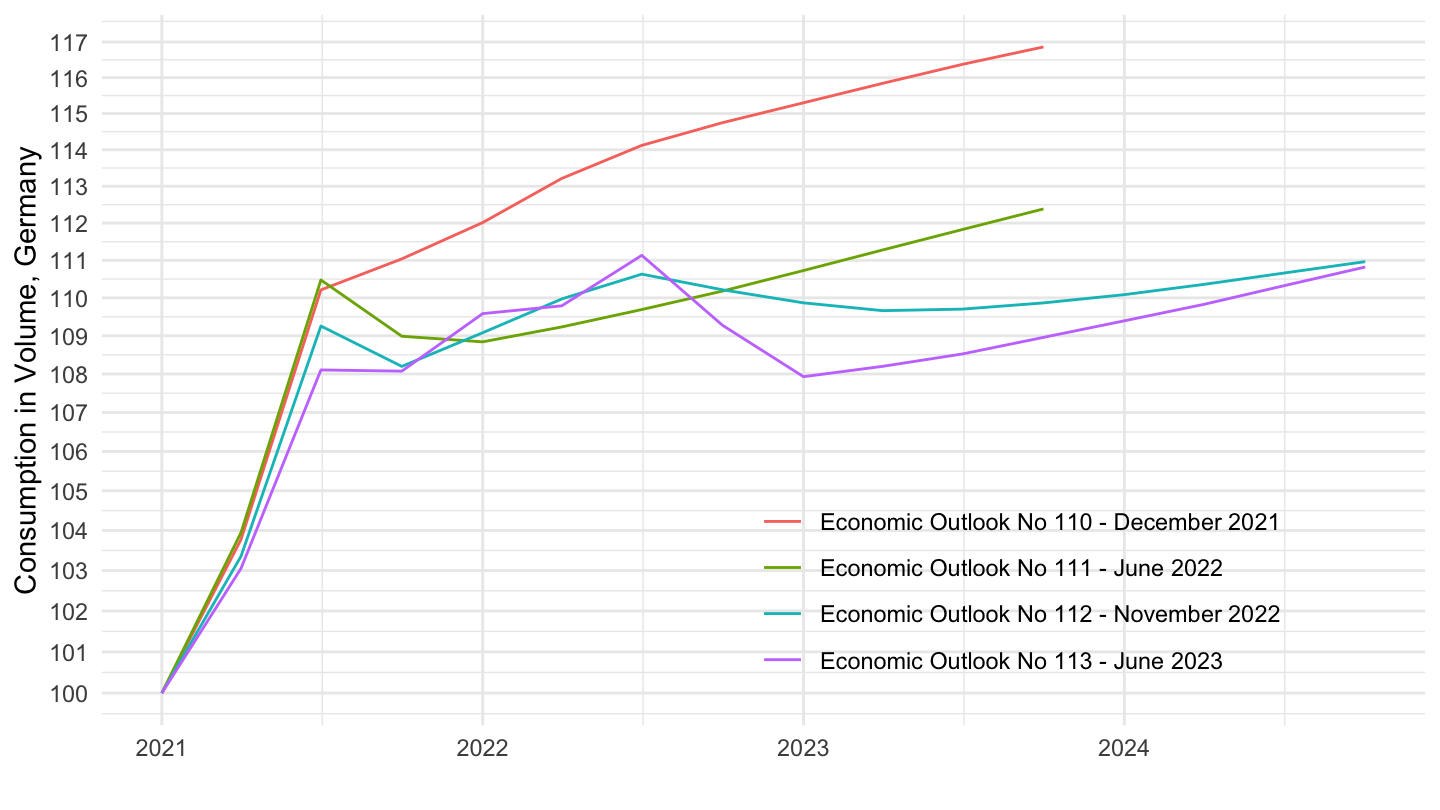
EO110_INTERNET |>
  mutate(vintage = "Economic Outlook No 110 - December 2021") |>
  bind_rows(EO111_INTERNET |>
              mutate(vintage = "Economic Outlook No 111 - June 2022")) |>
  bind_rows(EO112_INTERNET |>
              mutate(vintage = "Economic Outlook No 112 - November 2022")) |>
  bind_rows(EO113_INTERNET |>
              mutate(vintage = "Economic Outlook No 113 - June 2023")) |>
  filter(VARIABLE == "ITV",
         LOCATION == "DEU",
         FREQUENCY == "Q") |>
  quarter_to_date() |>
  filter(date >= as.Date("2021-01-01")) |>
  group_by(vintage) |>
  mutate(obsValue = 100*obsValue/obsValue[date == as.Date("2021-01-01")]) |>
  ggplot() + geom_line(aes(x = date, y = obsValue, color = vintage)) +
  xlab("") + ylab("Investment in Volume, Germany") + theme_minimal() +
  scale_x_date(breaks = seq(1920, 2100, 1) |> paste0("-01-01") |> as.Date(),
               labels = date_format("%Y")) +
  theme(legend.position = c(0.7, 0.2),
        legend.title = element_blank()) +
  scale_y_log10(breaks = seq(20, 200, 1))
EO110_INTERNET |>
  mutate(vintage = "2021-12") |>
  bind_rows(EO111_INTERNET |>
              mutate(vintage = "2022-06")) |>
  bind_rows(EO112_INTERNET |>
              mutate(vintage = "2022-11")) |>
  bind_rows(EO113_INTERNET |>
              mutate(vintage = "2023-06")) |>
  left_join(EO113_INTERNET_var$LOCATION, by = "LOCATION") |>
  filter(VARIABLE == "GDPV",
         obsTime == "2023-Q1",
         FREQUENCY == "Q") |>
  select(vintage, Location, obsValue) |>
  group_by(Location) |>
  mutate(obsValue = 100*obsValue/obsValue[vintage == "2021-12"]) |>
  spread(vintage, obsValue) |>
  arrange(`2023-06`) |>
print_table_conditional()EO113_INTERNET |>
filter(FREQUENCY == "A",
VARIABLE == "GAP",
LOCATION %in% c("DEU", "ESP", "GRC", "ITA")) |>
left_join(EO113_INTERNET_var$LOCATION, by = "LOCATION") |>
year_to_date() |>
select(Location, date, obsValue) |>
arrange(Location, date) |>
mutate(obsValue = obsValue/100) |>
add_flag_color("Location") |>
ggplot() +
geom_line(aes(x = date, y = obsValue, color = color)) +
theme_minimal() + scale_color_identity() + add_4flags +
scale_x_date(breaks = seq(1920, 2100, 5) |> paste0("-01-01") |> as.Date(),
labels = date_format("%Y")) +
scale_y_continuous(breaks = 0.01*seq(-60, 60, 5),
labels = scales::percent_format(accuracy = 1)) +
ylab("Output Gap (% of GDP)") + xlab("")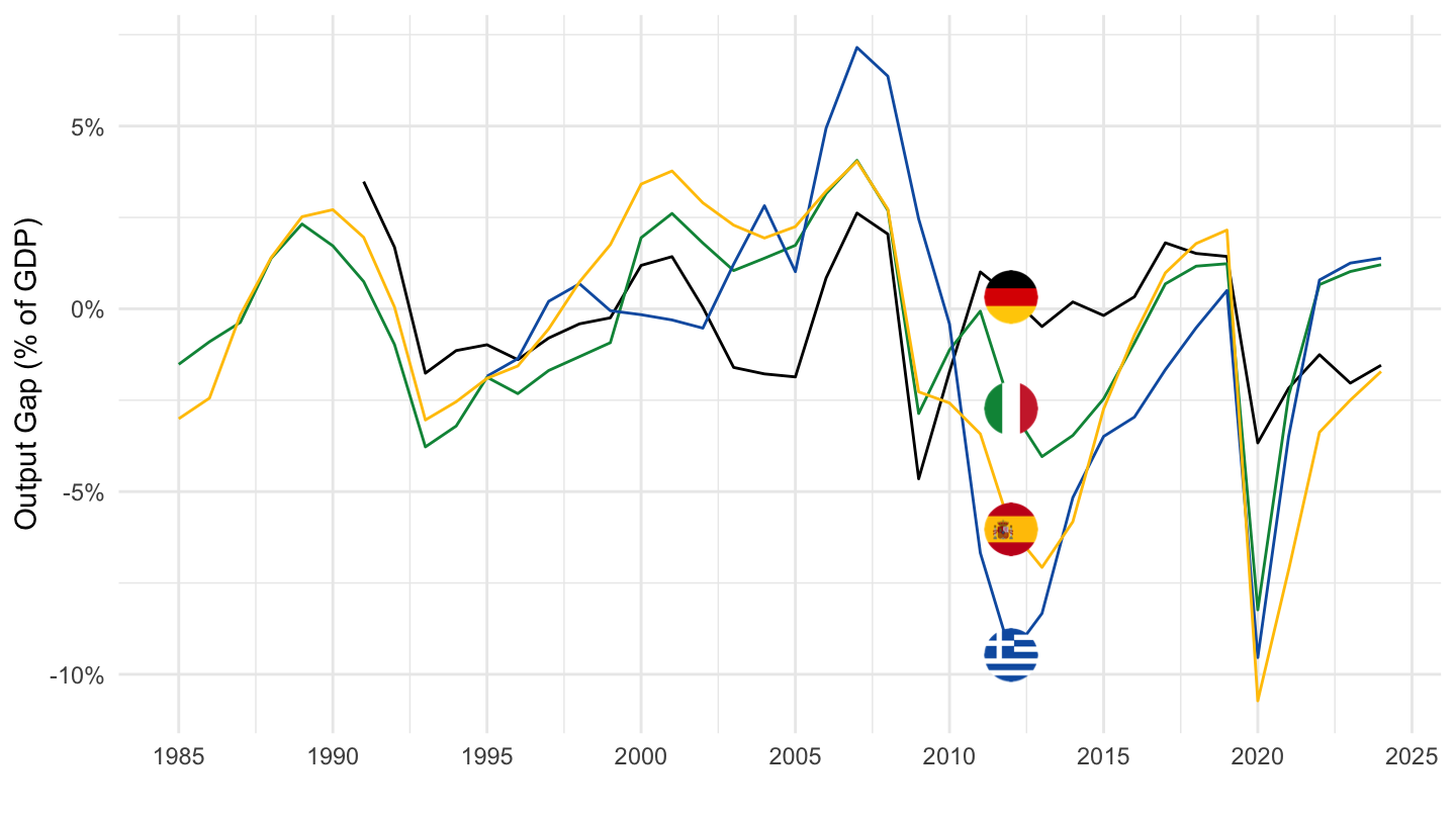
EO113_INTERNET |>
  filter(FREQUENCY == "A",
         VARIABLE == "GAP",
         LOCATION %in% c("CHE", "FRA", "DEU", "USA")) |>
  left_join(EO113_INTERNET_var$LOCATION, by = "LOCATION") |>
  year_to_date() |>
  select(Location, date, obsValue) |>
  arrange(Location, date) |>
  mutate(obsValue = obsValue/100) |>
  add_flag_color("Location") |>
  ggplot() +
  geom_line(aes(x = date, y = obsValue, color = color)) +
  theme_minimal() + scale_color_identity() + add_4flags +
  scale_x_date(breaks = seq(1920, 2100, 5) |> paste0("-01-01") |> as.Date(),
               labels = date_format("%Y")) +
  scale_y_continuous(breaks = 0.01*seq(-60, 60, 5),
                     labels = scales::percent_format(accuracy = 1)) +
  ylab("Output Gap (% of GDP)") + xlab("")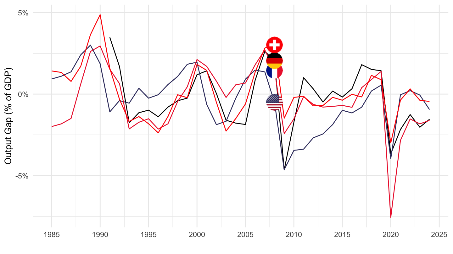
EO113_INTERNET |>
  filter(FREQUENCY == "Q",
         VARIABLE == "UNR",
         LOCATION %in% c("DEU", "ITA", "FRA", "USA")) |>
  left_join(EO113_INTERNET_var$LOCATION, by = "LOCATION") |>
  quarter_to_date() |>
  select(Location, date, obsValue) |>
  arrange(Location, date) |>
  mutate(obsValue = obsValue/100) |>
  add_flag_color("Location") |>
  ggplot() +
  geom_line(aes(x = date, y = obsValue, color = color)) +
  theme_minimal() + scale_color_identity() + add_4flags +
  scale_x_date(breaks = seq(1920, 2100, 5) |> paste0("-01-01") |> as.Date(),
               labels = date_format("%Y")) +
  scale_y_continuous(breaks = 0.01*seq(-60, 60, 1),
                     labels = scales::percent_format(accuracy = 1)) +
  ylab("Unemployment Rate (%)") + xlab("")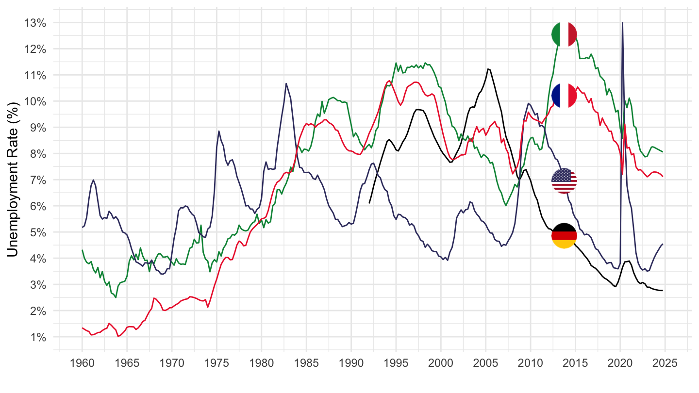
EO113_INTERNET |>
  filter(FREQUENCY == "Q",
         VARIABLE == "UNR",
         LOCATION %in% c("DEU", "ITA", "FRA", "USA")) |>
  left_join(EO113_INTERNET_var$LOCATION, by = "LOCATION") |>
  quarter_to_date() |>
  filter(date >= as.Date("1990-01-01")) |>
  select(Location, date, obsValue) |>
  arrange(Location, date) |>
  mutate(obsValue = obsValue/100) |>
  add_flag_color("Location") |>
  ggplot() +
  geom_line(aes(x = date, y = obsValue, color = color)) +
  theme_minimal() + scale_color_identity() + add_4flags +
  scale_x_date(breaks = seq(1920, 2100, 5) |> paste0("-01-01") |> as.Date(),
               labels = date_format("%Y")) +
  scale_y_continuous(breaks = 0.01*seq(-60, 60, 1),
                     labels = scales::percent_format(accuracy = 1)) +
  ylab("Unemployment Rate (%)") + xlab("")
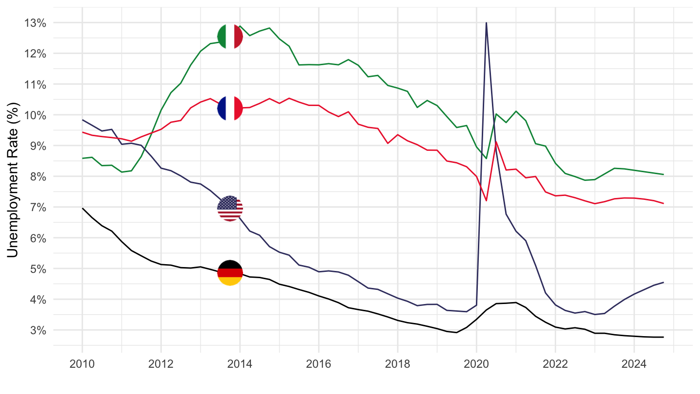
EO113_INTERNET |>
  filter(FREQUENCY == "Q",
         VARIABLE == "UNR",
         LOCATION %in% c("DEU", "ITA", "FRA", "USA")) |>
  left_join(EO113_INTERNET_var$LOCATION, by = "LOCATION") |>
  quarter_to_date() |>
  filter(date >= as.Date("2010-01-01")) |>
  select(Location, date, obsValue) |>
  arrange(Location, date) |>
  mutate(obsValue = obsValue/100) |>
  add_flag_color("Location") |>
  ggplot() +
  geom_line(aes(x = date, y = obsValue, color = color)) +
  theme_minimal() + scale_color_identity() + add_4flags +
  scale_x_date(breaks = seq(1920, 2100, 2) |> paste0("-01-01") |> as.Date(),
               labels = date_format("%Y")) +
  scale_y_continuous(breaks = 0.01*seq(-60, 60, 1),
                     labels = scales::percent_format(accuracy = 1)) +
  ylab("Unemployment Rate (%)") + xlab("")