2011
GGXWDG_GDP %>%
select(TIME_PERIOD, REF_AREA, GGXWDG_GDP = OBS_VALUE) %>%
left_join(IFR_BP6_USD, by = c("TIME_PERIOD", "REF_AREA")) %>%
year_to_date2 %>%
rename(iso2c = REF_AREA) %>%
left_join(NY.GDP.MKTP.CD %>%
mutate(date = as.Date(paste0(year, "-01-01"))) %>%
select(date, iso2c, NY.GDP.MKTP.CD),
by = c("date", "iso2c")) %>%
filter(date == as.Date("2011-01-01")) %>%
mutate(IFR_BP6_USD_GDP = -(10^(UNIT_MULT))*OBS_VALUE / NY.GDP.MKTP.CD) %>%
left_join(iso2c, by = "iso2c") %>%
ggplot(.) + theme_minimal() +
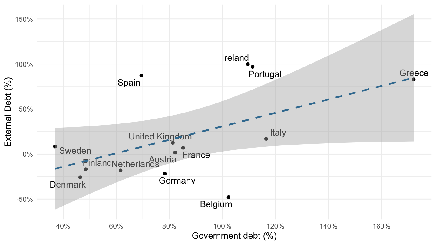
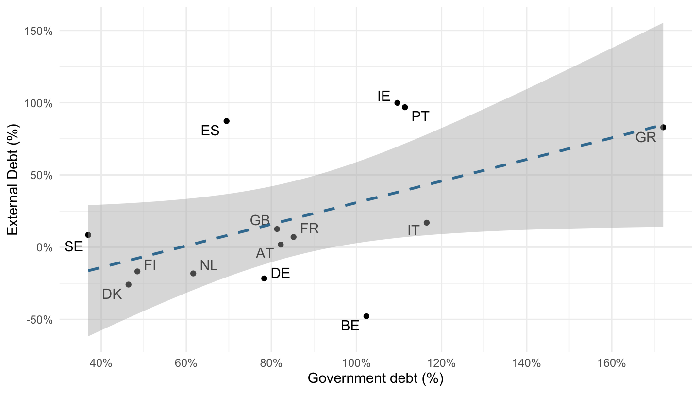
geom_point(aes(x = GGXWDG_GDP/100, y = IFR_BP6_USD_GDP)) +
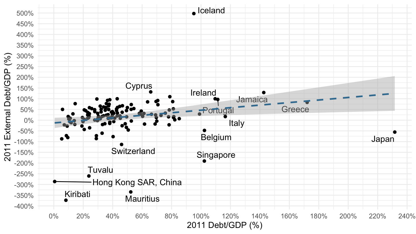
xlab("2011 Debt/GDP (%)") + ylab("2011 External Debt/GDP (%)") +
scale_x_continuous(breaks = 0.01*seq(-100, 600, 20),
labels = scales::percent_format(accuracy = 1)) +
scale_y_continuous(breaks = 0.01*seq(-600, 600, 50),
labels = scales::percent_format(accuracy = 1)) +
geom_text_repel(aes(x = GGXWDG_GDP/100, y = IFR_BP6_USD_GDP, label = Iso2c)) +
stat_smooth(aes(x = GGXWDG_GDP/100, y = IFR_BP6_USD_GDP),
linetype = 2, method = "lm", color = viridis(4)[2])
GGXWDG_GDP %>%
  select(TIME_PERIOD, REF_AREA, GGXWDG_GDP = OBS_VALUE) %>%
  left_join(IFR_BP6_USD, by = c("TIME_PERIOD", "REF_AREA")) %>%
  year_to_date2 %>%
  rename(iso2c = REF_AREA) %>%
  left_join(NY.GDP.MKTP.CD %>%
              mutate(date = as.Date(paste0(year, "-01-01"))) %>%
              select(date, iso2c, NY.GDP.MKTP.CD),
            by = c("date", "iso2c")) %>%
  filter(date == as.Date("2011-01-01")) %>%
  mutate(IFR_BP6_USD_GDP = -(10^(UNIT_MULT))*OBS_VALUE / NY.GDP.MKTP.CD) %>%
  left_join(iso2c, by = "iso2c") %>%
  lm(IFR_BP6_USD_GDP ~ GGXWDG_GDP, data = .) %>%
  summary
#
# Call:
# lm(formula = IFR_BP6_USD_GDP ~ GGXWDG_GDP, data = .)
#
# Residuals:
#     Min      1Q  Median      3Q     Max
# -3.6541 -0.1890  0.0849  0.3986  4.5374
#
# Coefficients:
#              Estimate Std. Error t value Pr(>|t|)
# (Intercept) -0.129081   0.122047  -1.058  0.29206
# GGXWDG_GDP   0.005943   0.002174   2.733  0.00708 **
# ---
# Signif. codes:  0 '***' 0.001 '**' 0.01 '*' 0.05 '.' 0.1 ' ' 1
#
# Residual standard error: 0.8253 on 139 degrees of freedom
#   (46 observations deleted due to missingness)
# Multiple R-squared:  0.05101, Adjusted R-squared:  0.04418
# F-statistic: 7.471 on 1 and 139 DF,  p-value: 0.007085