Error in readChar(con, 5L, useBytes = TRUE) :
  impossible d'ouvrir la connexion
Error in readChar(con, 5L, useBytes = TRUE) :
impossible d'ouvrir la connexionData - ECB
Error in readChar(con, 5L, useBytes = TRUE) :
impossible d'ouvrir la connexionError in readChar(con, 5L, useBytes = TRUE) :
impossible d'ouvrir la connexion| LAST_COMPILE |
|---|
| 2026-07-26 |
MNA %>%
  group_by(TIME_PERIOD) %>%
  summarise(Nobs = n()) %>%
  arrange(desc(TIME_PERIOD)) %>%
  head(1) %>%
print_table_conditional()| TIME_PERIOD | Nobs |
|---|---|
| 2026-Q2 | 2 |
MNA %>%
  left_join(STO, by = "STO") %>%
  group_by(STO, Sto) %>%
  summarise(Nobs = n()) %>%
  arrange(-Nobs) %>%
{if (is_html_output()) datatable(., filter = 'top', rownames = F) else .}MNA %>%
left_join(PRICES, by = "PRICES") %>%
group_by(PRICES, Prices) %>%
summarise(Nobs = n()) %>%
arrange(-Nobs) %>%
{if (is_html_output()) print_table(.) else .}| PRICES | Prices | Nobs |
|---|---|---|
| V | Current prices | 1255531 |
| LR | Chain linked volume (rebased) | 848838 |
| D | Deflator (index) | 389146 |
| _Z | Not applicable | 212926 |
| Y | Previous year prices | 191725 |
MNA %>%
  left_join(ADJUSTMENT, by = "ADJUSTMENT") %>%
  group_by(ADJUSTMENT, Adjustment) %>%
  summarise(Nobs = n()) %>%
  arrange(-Nobs) %>%
{if (is_html_output()) print_table(.) else .}| ADJUSTMENT | Adjustment | Nobs |
|---|---|---|
| N | Neither seasonally nor working day adjusted | 1447999 |
| Y | Working day and seasonally adjusted | 1234101 |
| S | Seasonally adjusted, not working day adjusted | 147323 |
| W | Working day adjusted, not seasonally adjusted | 68743 |
MNA %>%
  left_join(FREQ,  by = "FREQ") %>%
  group_by(FREQ, Freq) %>%
  summarise(Nobs = n()) %>%
  arrange(-Nobs) %>%
{if (is_html_output()) print_table(.) else .}| FREQ | Freq | Nobs |
|---|---|---|
| Q | Quarterly | 2597592 |
| A | Annual | 300574 |
MNA %>%
  left_join(REF_AREA,  by = "REF_AREA") %>%
  group_by(REF_AREA, Ref_area) %>%
  summarise(Nobs = n()) %>%
  arrange(-Nobs) %>%
{if (is_html_output()) datatable(., filter = 'top', rownames = F) else .}MNA %>%
left_join(COUNTERPART_AREA, by = "COUNTERPART_AREA") %>%
group_by(COUNTERPART_AREA, Counterpart_area) %>%
summarise(Nobs = n()) %>%
arrange(-Nobs) %>%
{if (is_html_output()) print_table(.) else .}| COUNTERPART_AREA | Counterpart_area | Nobs |
|---|---|---|
| W2 | Intra-Euro area not allocated | 1917737 |
| W0 | Intra-EU (changing composition) not allocated | 883016 |
| W1 | Gaza and Jericho | 97413 |
MNA %>%
  group_by(TITLE) %>%
  summarise(Nobs = n()) %>%
  arrange(-Nobs) %>%
{if (is_html_output()) datatable(., filter = 'top', rownames = F) else .}B1GQ %>%
ggplot + geom_line(aes(x = date, y = B1GQ)) +
theme_minimal() + xlab("") + ylab("") +
scale_y_log10(breaks = seq(0, 20000, 500),
labels = dollar_format(acc = 1, pre = "", su = "Bn€")) +
scale_x_date(breaks = as.Date(paste0(seq(1940, 2030, 2), "-01-01")),
labels = date_format("%Y"))
B1GQ %>%
  filter(date >= as.Date("1999-01-01")) %>%
  ggplot + geom_line(aes(x = date, y = B1GQ)) +
  theme_minimal() + xlab("") + ylab("") +
  scale_y_log10(breaks = seq(0, 20000, 1000),
                labels = dollar_format(acc = 1, pre = "", su = "Bn€")) +
  scale_x_date(breaks = as.Date(paste0(seq(1940, 2030, 2), "-01-01")),
               labels = date_format("%Y"))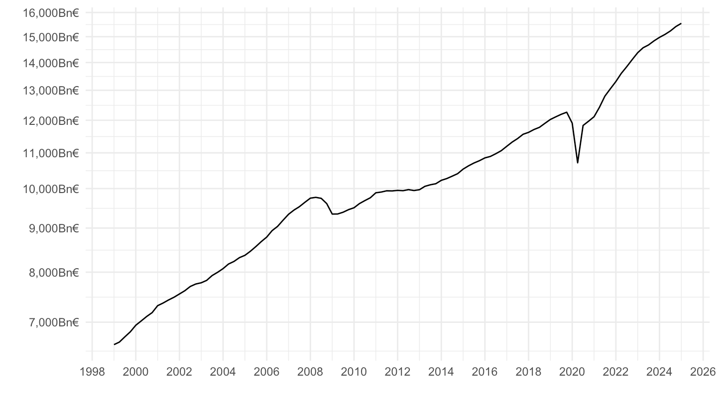
tibble(date = seq.Date(from = as.Date("1995-01-01"), to = Sys.Date(), "1 month")) %>%
  left_join(B1GQ %>% mutate(date = date + months(3)), by = "date") %>%
  mutate(B1GQ_i = spline(x = date, y = B1GQ, xout = date)$y) %>%
  gather(variable, value, -date) %>%
  filter(!is.na(value)) %>%
  ggplot + geom_line(aes(x = date, y = value, color = variable)) +
  theme_minimal() + xlab("") + ylab("") +
  theme(legend.position = c(0.25, 0.9),
        legend.title = element_blank()) +
  scale_y_log10(breaks = seq(0, 20000, 500),
                labels = dollar_format(acc = 1, pre = "", su = "Bn€")) +
  scale_x_date(breaks = as.Date(paste0(seq(1940, 2030, 2), "-01-01")),
               labels = date_format("%Y"))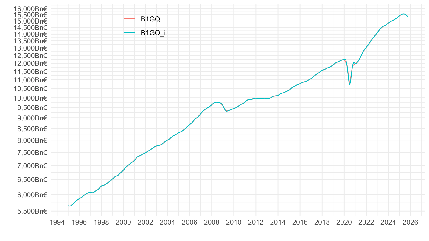
tibble(date = seq.Date(from = as.Date("1995-01-01"), to = Sys.Date(), "1 month")) %>%
  left_join(B1GQ %>% mutate(date = date + months(3)), by = "date") %>%
  mutate(B1GQ_i = spline(x = date, y = B1GQ, xout = date)$y) %>%
  gather(variable, value, -date) %>%
  filter(date >= as.Date("2010-01-01"),
         !is.na(value)) %>%
  ggplot + geom_line(aes(x = date, y = value, color = variable)) +
  theme_minimal() + xlab("") + ylab("") +
  scale_y_log10(breaks = seq(0, 20000, 500),
                labels = dollar_format(acc = 1, pre = "", su = "Bn€")) +
  theme(legend.position = c(0.25, 0.9),
        legend.title = element_blank()) +
  scale_x_date(breaks = as.Date(paste0(seq(1940, 2030, 2), "-01-01")),
               labels = date_format("%Y"))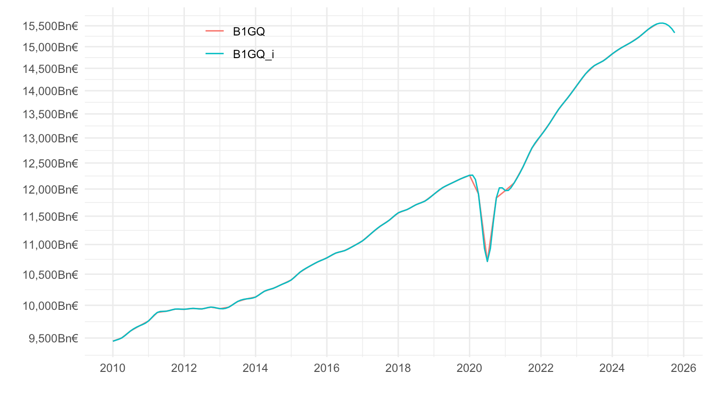
tibble(date = seq.Date(from = as.Date("1995-01-01"), to = Sys.Date(), "1 month")) %>%
  left_join(B1GQ %>% mutate(date = date + months(3)), by = "date") %>%
  mutate(B1GQ_i = spline(x = date, y = B1GQ, xout = date)$y) %>%
  gather(variable, value, -date) %>%
  filter(date >= as.Date("2019-01-01"),
         !is.na(value)) %>%
  ggplot + geom_line(aes(x = date, y = value, color = variable)) +
  theme_minimal() + xlab("") + ylab("") +
  scale_y_log10(breaks = seq(0, 20000, 500),
                labels = dollar_format(acc = 1, pre = "", su = "Bn€")) +
  theme(legend.position = c(0.25, 0.9),
        legend.title = element_blank()) +
  scale_x_date(breaks = as.Date(paste0(seq(1940, 2030, 1), "-01-01")),
               labels = date_format("%Y"))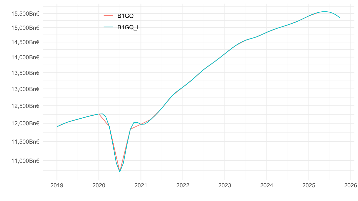
MNA %>%
  filter(ADJUSTMENT == "Y",
         REF_AREA == "I8",
         STO %in% c("P7", "P6"),
         # D: Deflator (index)
         PRICES == "D") %>%
  quarter_to_date() %>%
  ggplot() + theme_minimal() + ylab("") + xlab("") +
  geom_line(aes(x = date, y = OBS_VALUE/100, color = TITLE)) +

  scale_x_date(breaks = seq(1920, 2100, 2) %>% paste0("-01-01") %>% as.Date,
               labels = date_format("%Y")) +
  theme(legend.position = c(0.25, 0.9),
        legend.title = element_blank()) +
  scale_y_log10(breaks = 0.01*seq(0, 200, 5))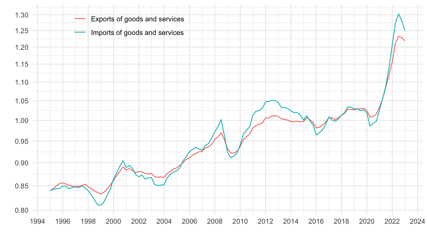
MNA %>%
  filter(ADJUSTMENT == "Y",
         REF_AREA == "I8",
         STO %in% c("P7", "P6"),
         # D: Deflator (index)
         PRICES == "D") %>%
  quarter_to_date() %>%
  filter(date >= as.Date("2000-01-01")) %>%
  ggplot() + theme_minimal() + ylab("") + xlab("") +
  geom_line(aes(x = date, y = OBS_VALUE/100, color = TITLE)) +

  scale_x_date(breaks = seq(1920, 2100, 2) %>% paste0("-01-01") %>% as.Date,
               labels = date_format("%Y")) +
  theme(legend.position = c(0.25, 0.9),
        legend.title = element_blank()) +
  scale_y_log10(breaks = 0.01*seq(0, 200, 5))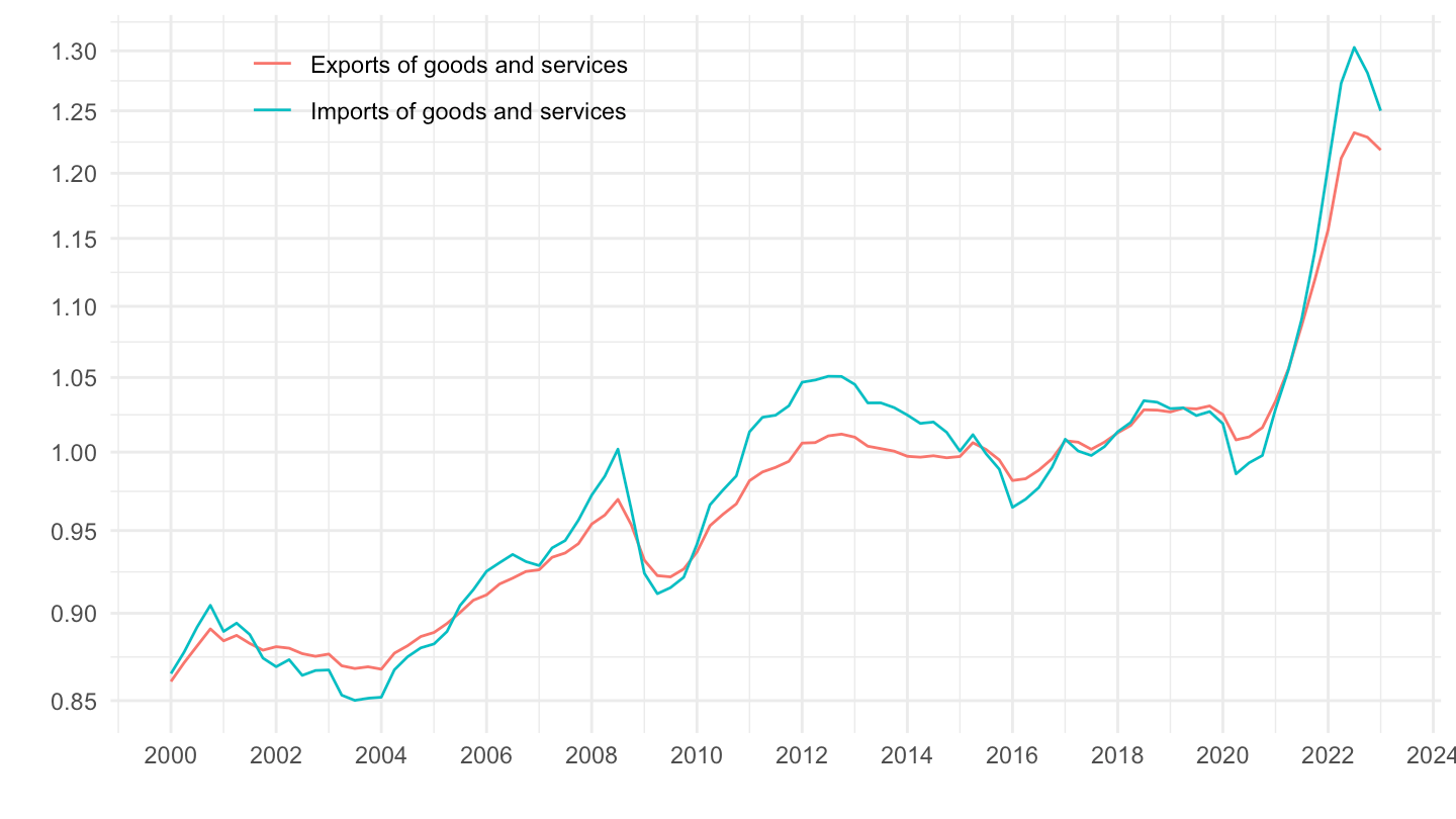
MNA %>%
  filter(ADJUSTMENT == "Y",
         REF_AREA == "I8",
         STO %in% c("P7", "P6"),
         # D: Deflator (index)
         PRICES == "D") %>%
  quarter_to_date() %>%
  filter(date >= as.Date("2009-01-01"),
         date <= as.Date("2014-12-31")) %>%
  group_by(TITLE) %>%
  ggplot() + theme_minimal() + ylab("") + xlab("") +
  geom_line(aes(x = date, y = OBS_VALUE, color = TITLE)) +

  scale_x_date(breaks = seq(1920, 2100, 1) %>% paste0("-01-01") %>% as.Date,
               labels = date_format("%Y")) +
  theme(legend.position = c(0.25, 0.9),
        legend.title = element_blank()) +
  scale_y_log10(breaks = seq(0, 200, 5))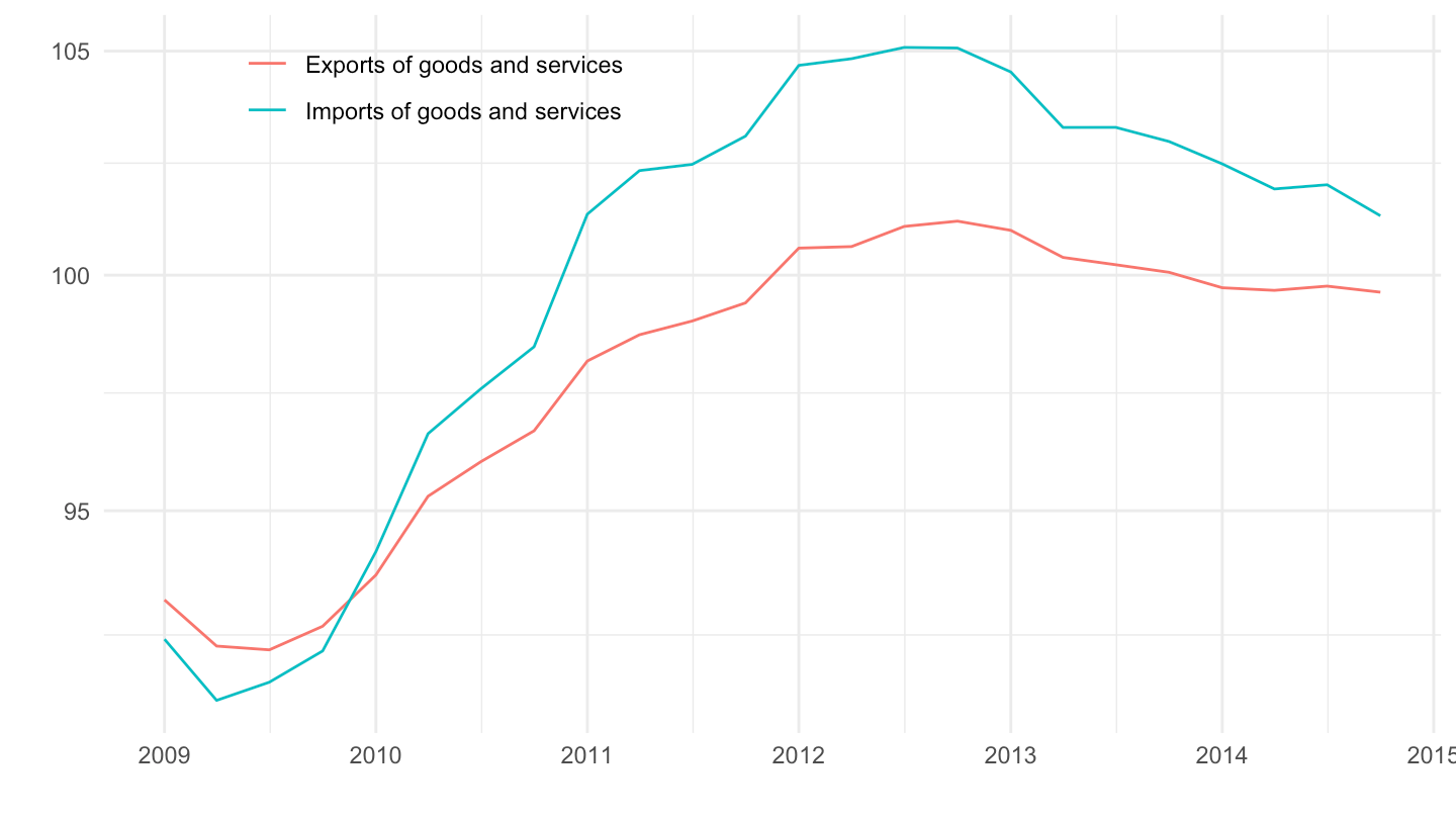
MNA %>%
  filter(ADJUSTMENT == "Y",
         REF_AREA == "I8",
         STO %in% c("P7", "P6"),
         # D: Deflator (index)
         PRICES == "D") %>%
  quarter_to_date() %>%
  group_by(TITLE) %>%
  mutate(OBS_VALUE = lead(log(OBS_VALUE), 4) - lag(log(OBS_VALUE), 4)) %>%
  filter(date >= as.Date("1997-01-01")) %>%
  ggplot() + theme_minimal() + ylab("") + xlab("") +
  geom_line(aes(x = date, y = OBS_VALUE, color = TITLE)) +

  scale_x_date(breaks = seq(1920, 2100, 2) %>% paste0("-01-01") %>% as.Date,
               labels = date_format("%Y")) +
  theme(legend.position = c(0.35, 0.9),
        legend.title = element_blank()) +
  scale_y_continuous(breaks = 0.01*seq(-100, 200, 2),
                     labels = percent_format(acc = 1))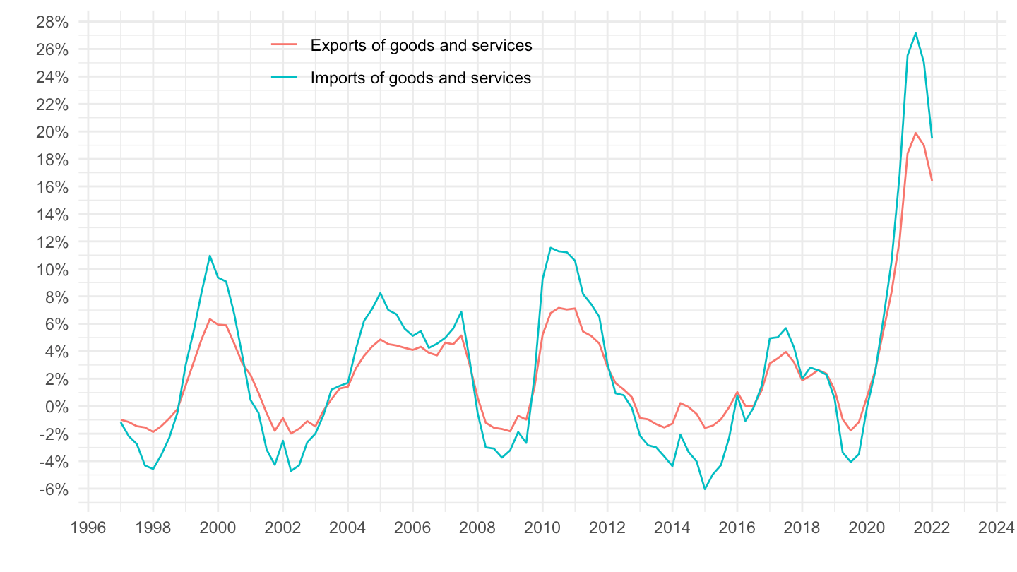
MNA %>%
  filter(ADJUSTMENT == "Y",
         REF_AREA == "I8",
         STO %in% c("P7", "P6"),
         # D: Deflator (index)
         PRICES == "D") %>%
  quarter_to_date() %>%
  group_by(TITLE) %>%
  mutate(OBS_VALUE = lead(log(OBS_VALUE), 4) - lag(log(OBS_VALUE), 4)) %>%
  filter(date >= as.Date("2000-01-01")) %>%
  ggplot() + theme_minimal() + ylab("") + xlab("") +
  geom_line(aes(x = date, y = OBS_VALUE, color = TITLE)) +

  scale_x_date(breaks = seq(1920, 2100, 2) %>% paste0("-01-01") %>% as.Date,
               labels = date_format("%Y")) +
  theme(legend.position = c(0.25, 0.9),
        legend.title = element_blank()) +
  scale_y_continuous(breaks = 0.01*seq(-100, 200, 1),
                     labels = percent_format(acc = 1))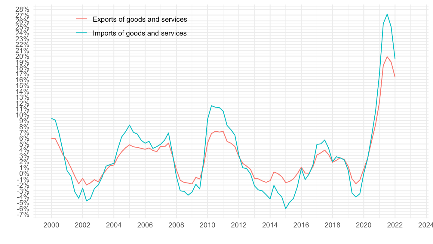
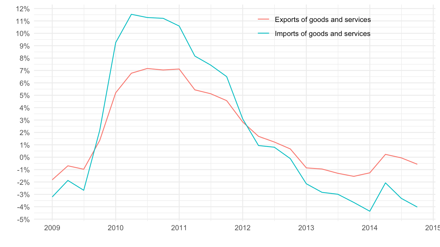
MNA %>%
  filter(ADJUSTMENT == "Y",
         REF_AREA == "I8",
         STO %in% c("P7", "P6"),
         # D: Deflator (index)
         PRICES == "D") %>%
  quarter_to_date() %>%
  group_by(TITLE) %>%
  mutate(OBS_VALUE = lead(log(OBS_VALUE), 4) - lag(log(OBS_VALUE), 4)) %>%
  filter(date >= as.Date("2009-01-01"),
         date <= as.Date("2014-12-31")) %>%
  ggplot() + theme_minimal() + ylab("") + xlab("") +
  geom_line(aes(x = date, y = OBS_VALUE, color = TITLE)) +

  scale_x_date(breaks = seq(1920, 2100, 1) %>% paste0("-01-01") %>% as.Date,
               labels = date_format("%Y")) +
  theme(legend.position = c(0.7, 0.9),
        legend.title = element_blank()) +
  scale_y_continuous(breaks = 0.01*seq(-100, 200, 1),
                     labels = percent_format(acc = 1))