Last data update: 12 sept. 2026, 09:59
Last compile: 07 oct. 2026, 04:23
CES |>
  group_by(Var, Var_label) |>
  summarise(Nobs = n()) |>
  arrange(-Nobs) |>
print_table_conditional()| Var | Var_label | Nobs |
|---|---|---|
| c1010 | Inflation perceptions over the previous 12 months (qualitative) | 675 |
| c1020 | Inflation perceptions over the previous 12 months (% change) | 675 |
| c1110 | Inflation expectations over the next 12 months (qualitative) | 675 |
| c1120 | Inflation expectations over the next 12 months (% change) | 675 |
| c1150 | Inflation expectations/uncertainty 12 months ahead (probabilistic bins) | 675 |
| c1210 | Inflation expectations 3 years ahead (qualitative) | 675 |
| c1220 | Inflation expectations 3 years ahead (% change) | 675 |
CES |>
  group_by(Breakdown, Breakdown_label) |>
  summarise(Nobs = n()) |>
  arrange(-Nobs) |>
print_table_conditional()| Breakdown | Breakdown_label | Nobs |
|---|---|---|
| Age | 18-34 years | 315 |
| Age | 35-54 years | 315 |
| Age | 55-70 years | 315 |
| Country | BE | 315 |
| Country | DE | 315 |
| Country | EA6 | 315 |
| Country | ES | 315 |
| Country | FR | 315 |
| Country | IT | 315 |
| Country | NL | 315 |
| Income | 1 | 315 |
| Income | 2 | 315 |
| Income | 3 | 315 |
| Income | 4 | 315 |
| Income | 5 | 315 |
CES |>
  filter(Breakdown == "Country") |>
  rename(geo = Breakdown_label) |>
  left_join(geo, by = "geo") |>
  group_by(geo, Geo) |>
  summarise(Nobs = n()) |>
  arrange(-Nobs) |>
print_table_conditional()| geo | Geo | Nobs |
|---|---|---|
| BE | Belgium | 315 |
| DE | Germany | 315 |
| EA6 | NA | 315 |
| ES | Spain | 315 |
| FR | France | 315 |
| IT | Italy | 315 |
| NL | Netherlands | 315 |
CES |>
  wave_to_date() |>
  group_by(date) |>
  summarise(Nobs = n()) |>
  arrange(desc(date)) |>
print_table_conditional()CES |>
wave_to_date() |>
filter(Breakdown == "Wave",
Var %in% c("c1020", "c1120", "c1220")) |>
transmute(date, Var_label, OBS_VALUE = Mean/100) |>
ggplot() + geom_line(aes(x = date, y = OBS_VALUE, color = Var_label)) +
theme_minimal() + xlab("") + ylab("Mean (%)") +
scale_x_date(breaks = seq.Date(as.Date("2019-12-01"), Sys.Date(), "2 months"),
labels = date_format("%b %Y")) +
scale_y_continuous(breaks = 0.01*seq(-20, 20, 1),
labels = percent_format(a = 1)) +
theme(legend.position = c(0.33, 0.90),
axis.text.x = element_text(angle = 45, vjust = 1, hjust = 1),
legend.title = element_blank())
CES |>
  wave_to_date() |>
  filter(Breakdown == "Wave",
         Var %in% c("c1020", "c1120", "c1220")) |>
  transmute(date, Var_label, OBS_VALUE = Median/100) |>
  ggplot() + geom_line(aes(x = date, y = OBS_VALUE, color = Var_label)) +
  theme_minimal() + xlab("") + ylab("Median (%)") +
  scale_x_date(breaks = seq.Date(as.Date("2019-12-01"), Sys.Date(), "2 months"),
               labels = date_format("%b %Y")) +
  scale_y_continuous(breaks = 0.01*seq(-20, 20, 1),
                     labels = percent_format(a = 1)) +
  theme(legend.position = c(0.33, 0.90),
        axis.text.x = element_text(angle = 45, vjust = 1, hjust = 1),
        legend.title = element_blank())
CES |>
  wave_to_date() |>
  filter(Breakdown == "Wave",
         Var %in% c("c1010", "c1110", "c1210")) |>
  transmute(date, Var_label, OBS_VALUE = Net_perc/100) |>
  ggplot() + geom_line(aes(x = date, y = OBS_VALUE, color = Var_label)) +
  theme_minimal() + xlab("") + ylab("Net_perc (%)") +
  scale_x_date(breaks = seq.Date(as.Date("2019-12-01"), Sys.Date(), "2 months"),
               labels = date_format("%b %Y")) +
  scale_y_continuous(breaks = 0.01*seq(-20, 100, 5),
                     labels = percent_format(a = 1)) +
  theme(legend.position = c(0.33, 0.90),
        axis.text.x = element_text(angle = 45, vjust = 1, hjust = 1),
        legend.title = element_blank())
CES |>
  wave_to_date() |>
  filter(Breakdown == "Wave",
         Var %in% c("c1010", "c1110", "c1210")) |>
  transmute(date, Var_label, OBS_VALUE = Net_perc/100) |>
  ggplot() + geom_line(aes(x = date, y = OBS_VALUE, color = Var_label)) +
  theme_minimal() + xlab("") + ylab("Up (%)") +
  scale_x_date(breaks = seq.Date(as.Date("2019-12-01"), Sys.Date(), "2 months"),
               labels = date_format("%b %Y")) +
  scale_y_continuous(breaks = 0.01*seq(-20, 100, 5),
                     labels = percent_format(a = 1)) +
  theme(legend.position = c(0.33, 0.90),
        axis.text.x = element_text(angle = 45, vjust = 1, hjust = 1),
        legend.title = element_blank())
CES |>
  wave_to_date() |>
  filter(Breakdown == "Wave",
         Var %in% c("c1010", "c1110", "c1210")) |>
  transmute(date, Var_label, OBS_VALUE = Down/100) |>
  ggplot() + geom_line(aes(x = date, y = OBS_VALUE, color = Var_label)) +
  theme_minimal() + xlab("") + ylab("Up (%)") +
  scale_x_date(breaks = seq.Date(as.Date("2019-12-01"), Sys.Date(), "2 months"),
               labels = date_format("%b %Y")) +
  scale_y_continuous(breaks = 0.01*seq(-20, 100, 1),
                     labels = percent_format(a = 1)) +
  theme(legend.position = c(0.33, 0.90),
        axis.text.x = element_text(angle = 45, vjust = 1, hjust = 1),
        legend.title = element_blank())
CES |>
  wave_to_date() |>
  filter(Breakdown == "Country",
         Var == "c1020") |>
  rename(geo = Breakdown_label) |>
  left_join(geo, by = "geo") |>
  add_flag_color("Geo") |>
  mutate(OBS_VALUE = Mean/100) |>
  rename(Ref_area = Geo) |>
  ggplot() + geom_line(aes(x = date, y = OBS_VALUE, color = color)) +
  theme_minimal() + xlab("") + ylab("Inflation expectations over the next 12 months\n% change, Mean") +
  scale_x_date(breaks = seq.Date(as.Date("2019-12-01"), Sys.Date(), "2 months"),
               labels = date_format("%b %Y")) +
  scale_y_continuous(breaks = 0.01*seq(-20, 20, 1),
                     labels = percent_format(a = 1)) +
  scale_color_identity() + add_flags +
  theme(legend.position = c(0.75, 0.90),
        axis.text.x = element_text(angle = 45, vjust = 1, hjust = 1),
        legend.title = element_blank())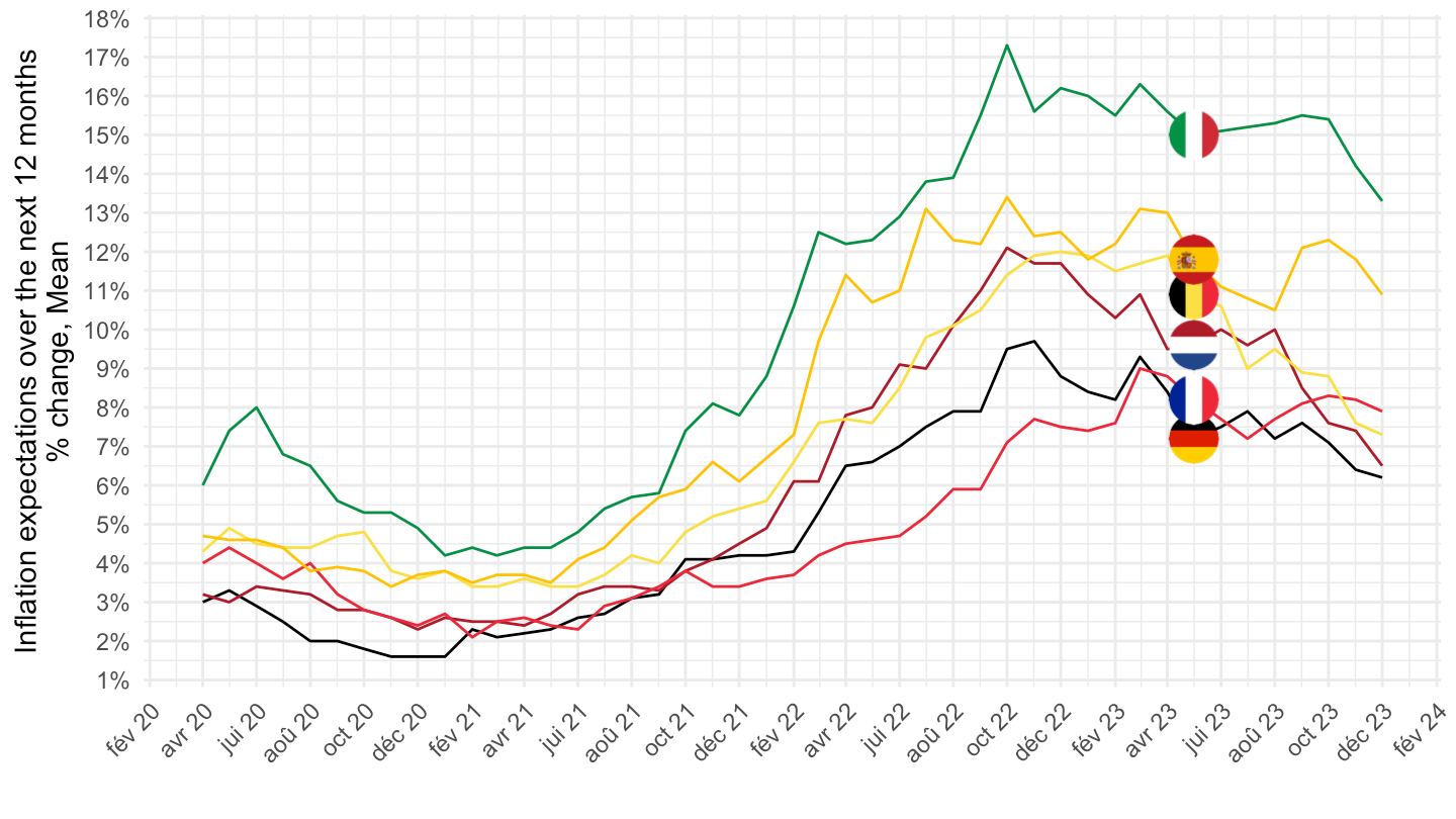
CES |>
  wave_to_date() |>
  filter(Breakdown == "Country",
         Var == "c1020") |>
  rename(geo = Breakdown_label) |>
  left_join(geo, by = "geo") |>
  add_flag_color("Geo") |>
  mutate(OBS_VALUE = Mean/100) |>
  filter(date >= as.Date("2021-10-01")) |>
  rename(Ref_area = Geo) |>
  ggplot() + geom_line(aes(x = date, y = OBS_VALUE, color = color)) +
  theme_minimal() + xlab("") + ylab("Inflation expectations over the next 12 months\n% change, Mean") +
  scale_x_date(breaks = seq.Date(as.Date("2019-12-01"), Sys.Date(), "1 month"),
               labels = date_format("%b %Y")) +
  scale_y_continuous(breaks = 0.01*seq(-20, 20, 1),
                     labels = percent_format(a = 1)) +
  scale_color_identity() + add_flags +
  theme(legend.position = c(0.75, 0.90),
        axis.text.x = element_text(angle = 45, vjust = 1, hjust = 1),
        legend.title = element_blank())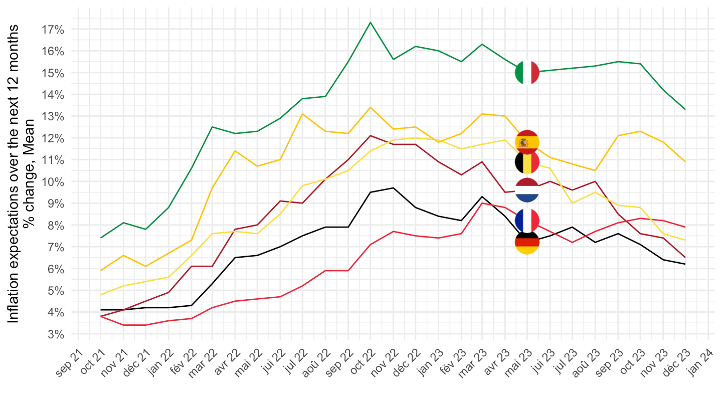
CES |>
  wave_to_date() |>
  filter(Breakdown == "Country",
         Var == "c1020") |>
  rename(geo = Breakdown_label) |>
  left_join(geo, by = "geo") |>
  add_flag_color("Geo") |>
  mutate(OBS_VALUE = Median/100) |>
  rename(Ref_area = Geo) |>
  ggplot() + geom_line(aes(x = date, y = OBS_VALUE, color = color)) +
  theme_minimal() + xlab("") + ylab("Inflation expectations over the next 12 months\n% change, Median") +
  scale_x_date(breaks = seq.Date(as.Date("2019-12-01"), Sys.Date(), "2 months"),
               labels = date_format("%b %Y")) +
  scale_y_continuous(breaks = 0.01*seq(-20, 20, 1),
                     labels = percent_format(a = 1)) +
  scale_color_identity() + add_flags +
  theme(legend.position = c(0.75, 0.90),
        axis.text.x = element_text(angle = 45, vjust = 1, hjust = 1),
        legend.title = element_blank())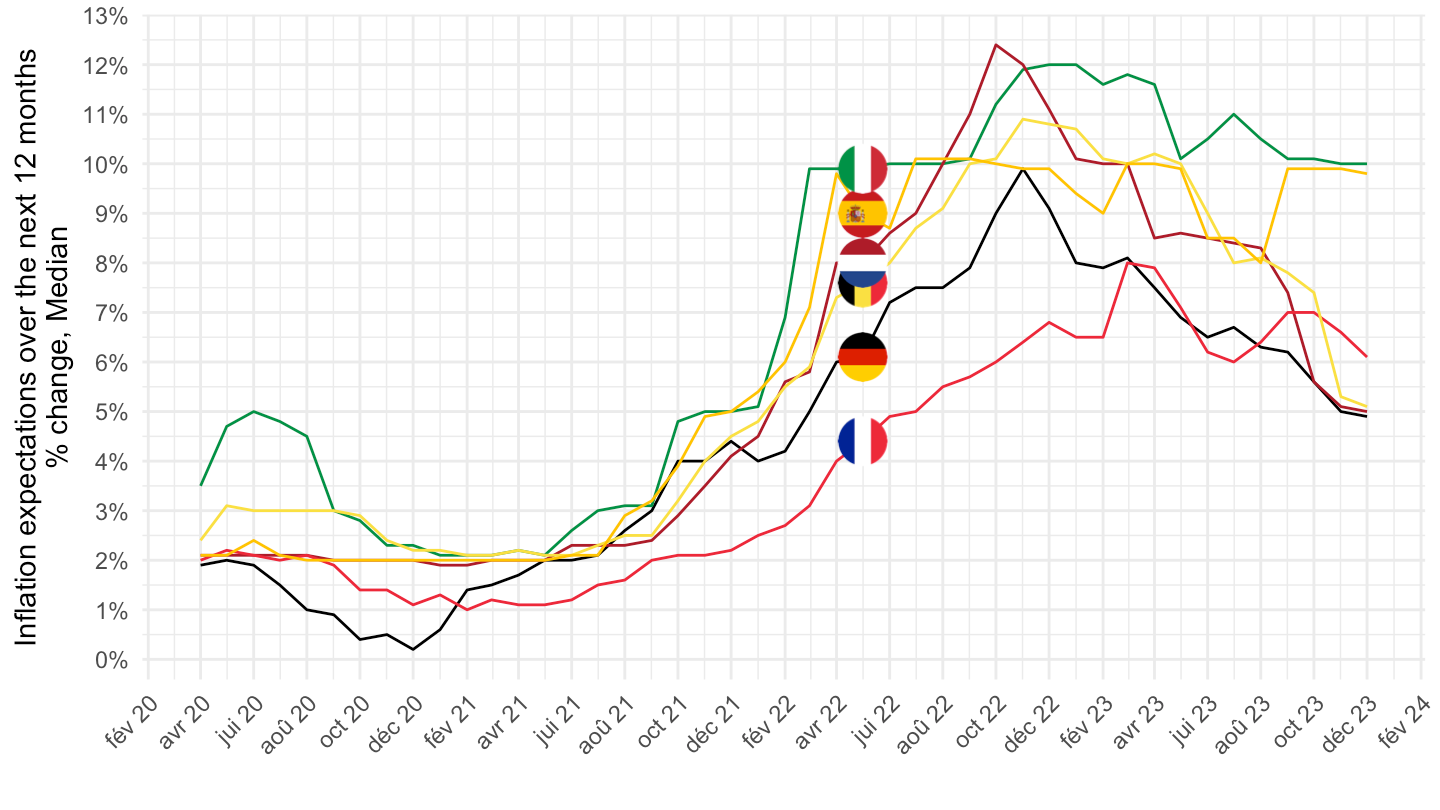
CES |>
  wave_to_date() |>
  filter(Breakdown == "Country",
         Var == "c1020") |>
  rename(geo = Breakdown_label) |>
  left_join(geo, by = "geo") |>
  add_flag_color("Geo") |>
  mutate(OBS_VALUE = Median/100) |>
  filter(date >= as.Date("2021-10-01")) |>
  rename(Ref_area = Geo) |>
  ggplot() + geom_line(aes(x = date, y = OBS_VALUE, color = color)) +
  theme_minimal() + xlab("") + ylab("Inflation expectations over the next 12 months\n% change, Median") +
  scale_x_date(breaks = seq.Date(as.Date("2019-12-01"), Sys.Date(), "1 month"),
               labels = date_format("%b %Y")) +
  scale_y_continuous(breaks = 0.01*seq(-20, 20, 1),
                     labels = percent_format(a = 1)) +
  scale_color_identity() + add_flags +
  theme(legend.position = c(0.75, 0.90),
        axis.text.x = element_text(angle = 45, vjust = 1, hjust = 1),
        legend.title = element_blank())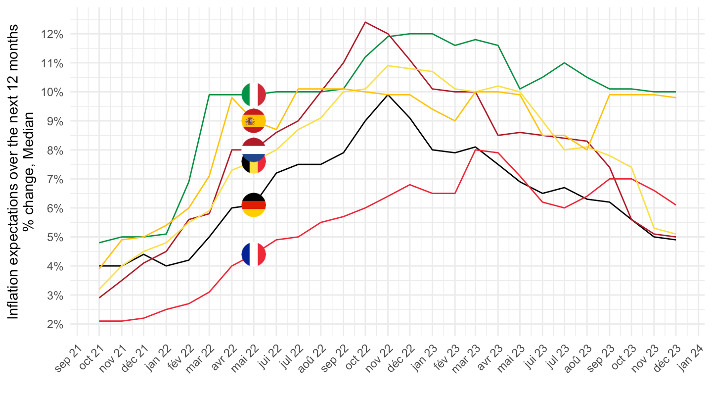
CES |>
  wave_to_date() |>
  filter(Breakdown == "Country",
         Var == "c1220") |>
  rename(geo = Breakdown_label) |>
  left_join(geo, by = "geo") |>
  add_flag_color("Geo") |>
  mutate(OBS_VALUE = Mean/100) |>
  rename(Ref_area = Geo) |>
  ggplot() + geom_line(aes(x = date, y = OBS_VALUE, color = color)) +
  theme_minimal() + xlab("") + ylab("Inflation expectations 3 years ahead\n% change, Mean") +
  scale_x_date(breaks = seq.Date(as.Date("2019-12-01"), Sys.Date(), "2 months"),
               labels = date_format("%b %Y")) +
  scale_y_continuous(breaks = 0.01*seq(-20, 20, 1),
                     labels = percent_format(a = 1)) +
  scale_color_identity() + add_flags +
  theme(legend.position = c(0.75, 0.90),
        axis.text.x = element_text(angle = 45, vjust = 1, hjust = 1),
        legend.title = element_blank())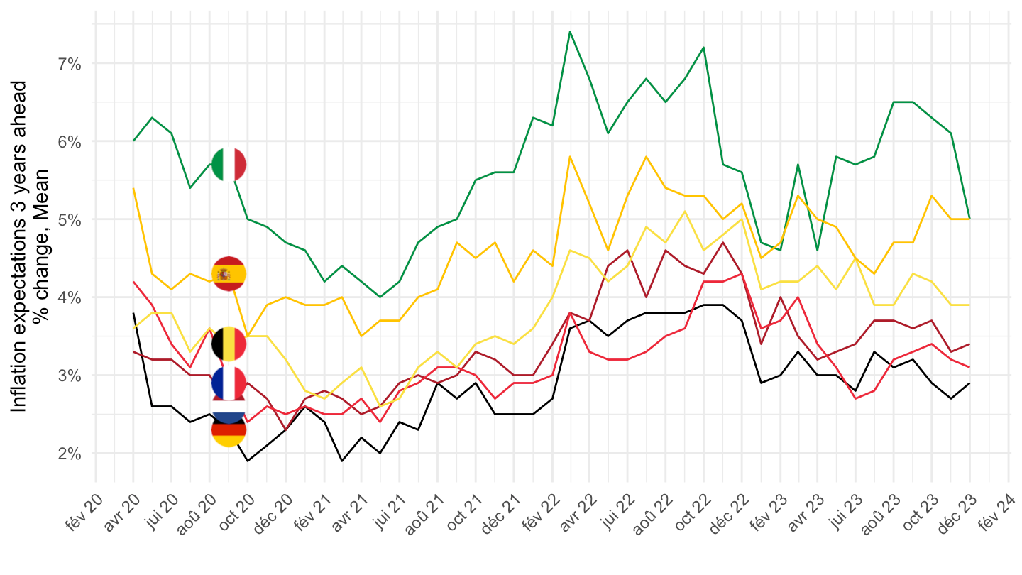
CES |>
  wave_to_date() |>
  filter(Breakdown == "Country",
         Var == "c1220",
         date >= as.Date("2021-10-01")) |>
  rename(geo = Breakdown_label) |>
  left_join(geo, by = "geo") |>
  add_flag_color("Geo") |>
  mutate(OBS_VALUE = Mean/100) |>
  rename(Ref_area = Geo) |>
  ggplot() + geom_line(aes(x = date, y = OBS_VALUE, color = color)) +
  theme_minimal() + xlab("") + ylab("Inflation expectations 3 years ahead\n% change, Mean") +
  scale_x_date(breaks = seq.Date(as.Date("2019-12-01"), Sys.Date(), "1 month"),
               labels = date_format("%b %Y")) +
  scale_y_continuous(breaks = 0.01*seq(-20, 20, 1),
                     labels = percent_format(a = 1)) +
  scale_color_identity() + add_flags +
  theme(legend.position = c(0.75, 0.90),
        axis.text.x = element_text(angle = 45, vjust = 1, hjust = 1),
        legend.title = element_blank())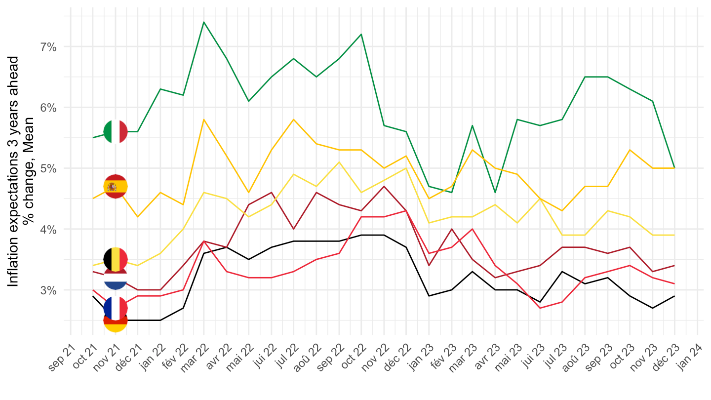
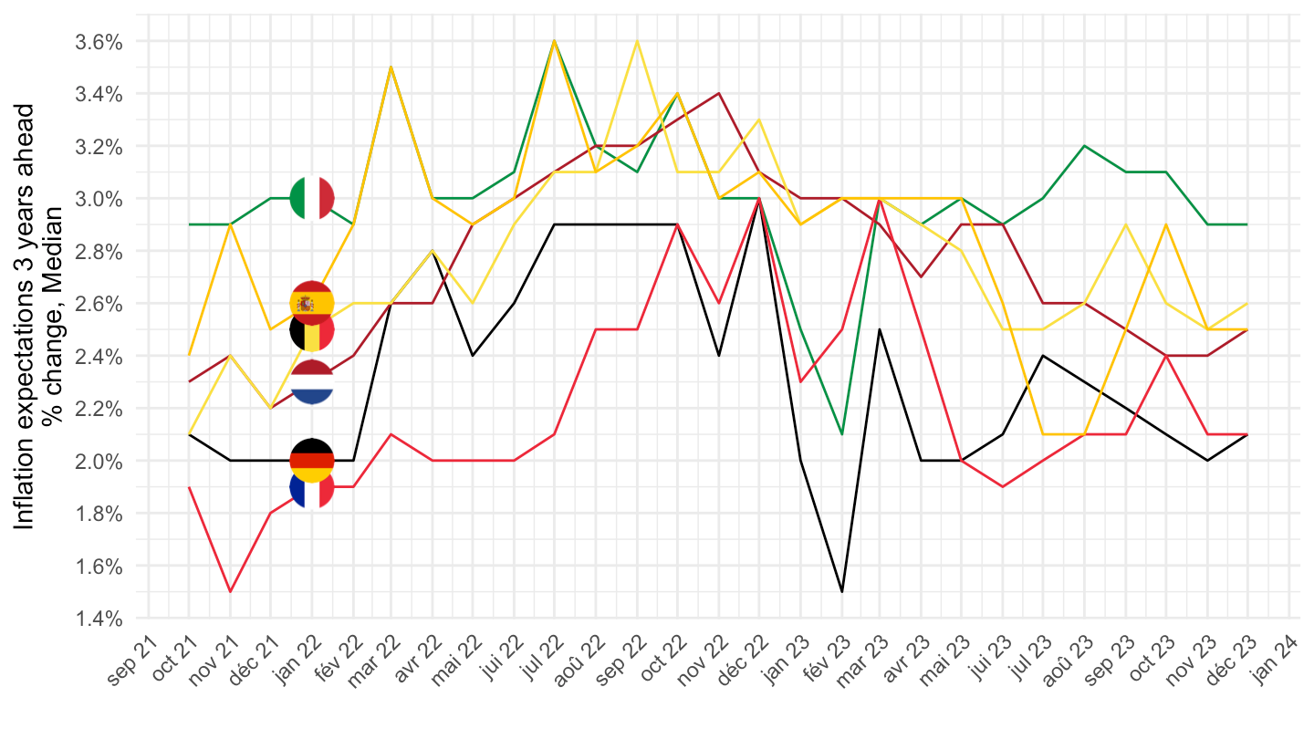
CES |>
  wave_to_date() |>
  filter(Breakdown == "Country",
         Var == "c1220") |>
  rename(geo = Breakdown_label) |>
  left_join(geo, by = "geo") |>
  add_flag_color("Geo") |>
  mutate(OBS_VALUE = Median/100) |>
  rename(Ref_area = Geo) |>
  ggplot() + geom_line(aes(x = date, y = OBS_VALUE, color = color)) +
  theme_minimal() + xlab("") + ylab("Inflation expectations 3 years ahead\n% change, Median") +
  scale_x_date(breaks = seq.Date(as.Date("2019-12-01"), Sys.Date(), "2 months"),
               labels = date_format("%b %Y")) +
  scale_y_continuous(breaks = 0.01*seq(-20, 20, .2),
                     labels = percent_format(a = .1)) +
  scale_color_identity() + add_flags +
  theme(legend.position = c(0.75, 0.90),
        axis.text.x = element_text(angle = 45, vjust = 1, hjust = 1),
        legend.title = element_blank())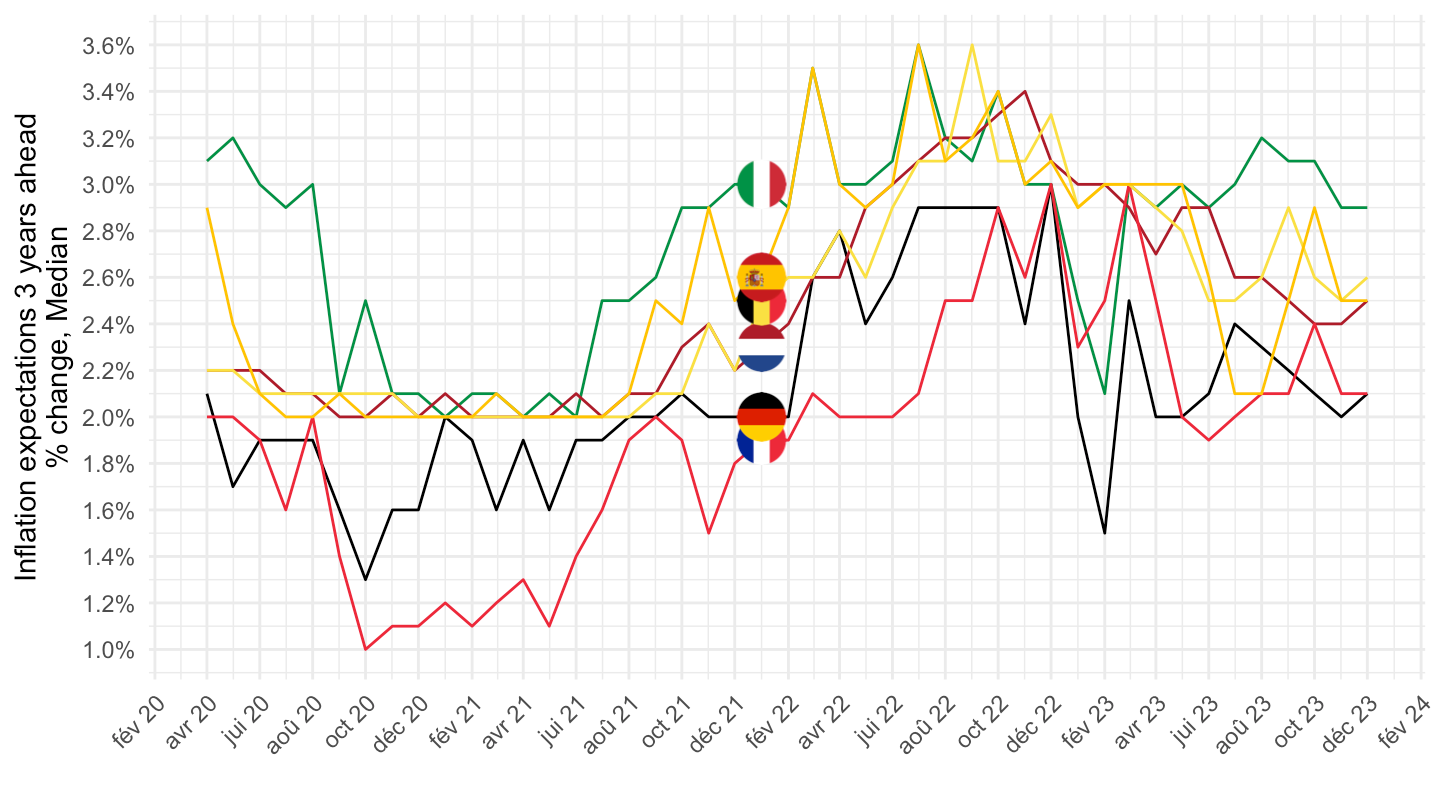
CES |>
  wave_to_date() |>
  filter(Breakdown == "Country",
         Var == "c1220",
         date >= as.Date("2021-10-01")) |>
  rename(geo = Breakdown_label) |>
  left_join(geo, by = "geo") |>
  add_flag_color("Geo") |>
  mutate(OBS_VALUE = Median/100) |>
  rename(Ref_area = Geo) |>
  ggplot() + geom_line(aes(x = date, y = OBS_VALUE, color = color)) +
  theme_minimal() + xlab("") + ylab("Inflation expectations 3 years ahead\n% change, Median") +
  scale_x_date(breaks = seq.Date(as.Date("2019-12-01"), Sys.Date(), "1 month"),
               labels = date_format("%b %Y")) +
  scale_y_continuous(breaks = 0.01*seq(-20, 20, .2),
                     labels = percent_format(a = .1)) +
  scale_color_identity() + add_flags +
  theme(legend.position = c(0.75, 0.90),
        axis.text.x = element_text(angle = 45, vjust = 1, hjust = 1),
        legend.title = element_blank())