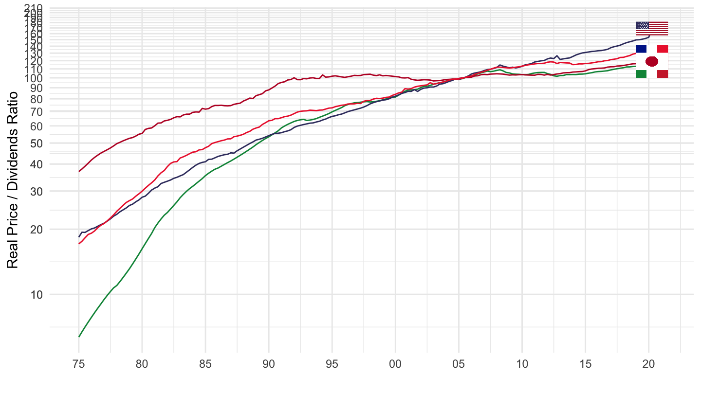
Last observation: Q2 2021 (N = 108)
First observation: Q1 1975 (N = 108)
Last data update: 01 août 2026, 21:07
Last compile: 10 oct. 2026, 00:11
dallas_fed |>
  left_join(variable, by = "variable") |>
  group_by(variable, Variable) |>
  summarise(Nobs = n()) |>
print_table_conditional()| variable | Variable | Nobs |
|---|---|---|
| HPI | House Prices (Dallas Fed) | 5022 |
| PDI | Price / Dividend Ratio | 5022 |
| RHPI | Real House Prices (Dallas Fed) | 5022 |
| RPDI | Real Price / Dividend Ratio | 5022 |
dallas_fed |>
  group_by(countryname) |>
  summarise(Nobs = n()) |>
  mutate(Flag = gsub(" ", "-", str_to_lower(gsub(" ", "-", countryname))),
         Flag = paste0('<img src="../../icon/flag/vsmall/', Flag, '.png" alt="Flag">')) |>
  select(Flag, everything()) %>%
{if (is_html_output()) datatable(., filter = 'top', rownames = F, escape = F) else .}dallas_fed |>
group_by(date) |>
summarise(Nobs = n()) |>
arrange(desc(date)) |>
print_table_conditional()dallas_fed |>
filter(countryname %in% c("Italy", "France", "United States"),
variable == "HPI") |>
add_flag_color("countryname") |>
ggplot() + theme_minimal() + xlab("") + ylab("Real House Prices") +
geom_line(aes(x = date, y = value, color = color)) +
scale_color_identity() + add_3flags +
scale_x_date(breaks = seq(1920, 2100, 5) |> paste0("-01-01") |> as.Date(),
labels = date_format("%Y")) +
scale_y_log10(breaks = c(seq(0, 500, 10), seq(10, 50, 10))) +
theme(legend.position = c(0.25, 0.8),
legend.title = element_blank())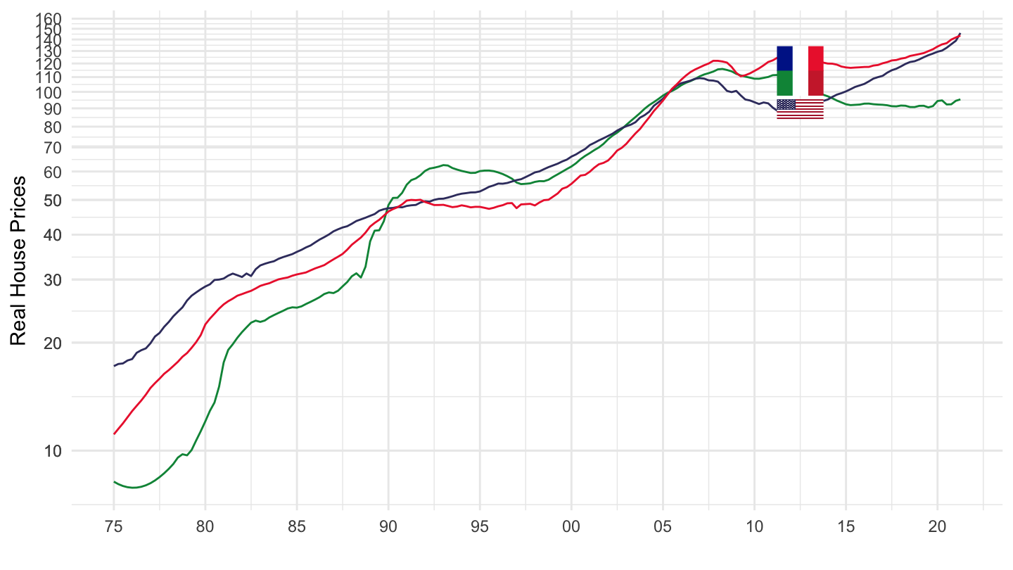
dallas_fed |>
  filter(countryname %in% c("Italy", "France", "United States", "Japan"),
         variable == "HPI") |>
  add_flag_color("countryname") |>
  ggplot() + theme_minimal() + xlab("") + ylab("Real House Prices") +
  geom_line(aes(x = date, y = value, color = color)) +
  scale_color_identity() + add_4flags +
  scale_x_date(breaks = seq(1920, 2100, 5) |> paste0("-01-01") |> as.Date(),
               labels = date_format("%Y")) +
  scale_y_log10(breaks = c(seq(0, 500, 10), seq(10, 50, 10))) +
  theme(legend.position = c(0.25, 0.8),
        legend.title = element_blank())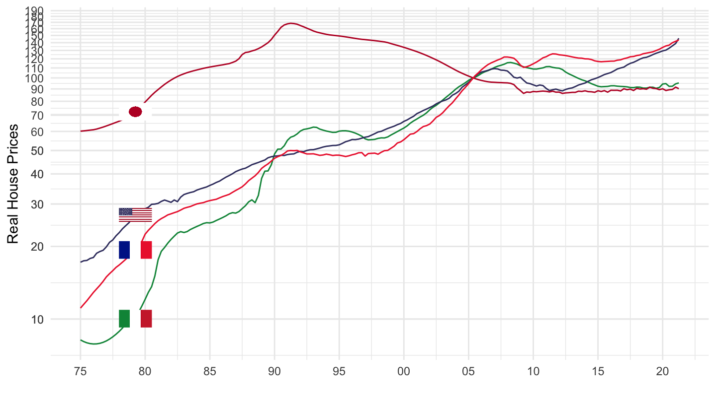
dallas_fed |>
  filter(countryname %in% c("United States", "France"),
         variable == "RHPI") |>
  add_flag_color("countryname") |>
  group_by(countryname) |>
  mutate(value = 100*value/value[date == as.Date("1997-01-01")]) |>
  ggplot() + theme_minimal() + xlab("") + ylab("Real House Prices (1997 = 100)") +
  geom_line(aes(x = date, y = value, color = color)) +
  scale_color_identity() + add_2flags +
  scale_x_date(breaks = seq(1920, 2100, 5) |> paste0("-01-01") |> as.Date(),
               labels = date_format("%Y")) +
  scale_y_log10(breaks = c(seq(0, 500, 10), seq(10, 50, 10))) +
  theme(legend.position = c(0.25, 0.8),
        legend.title = element_blank())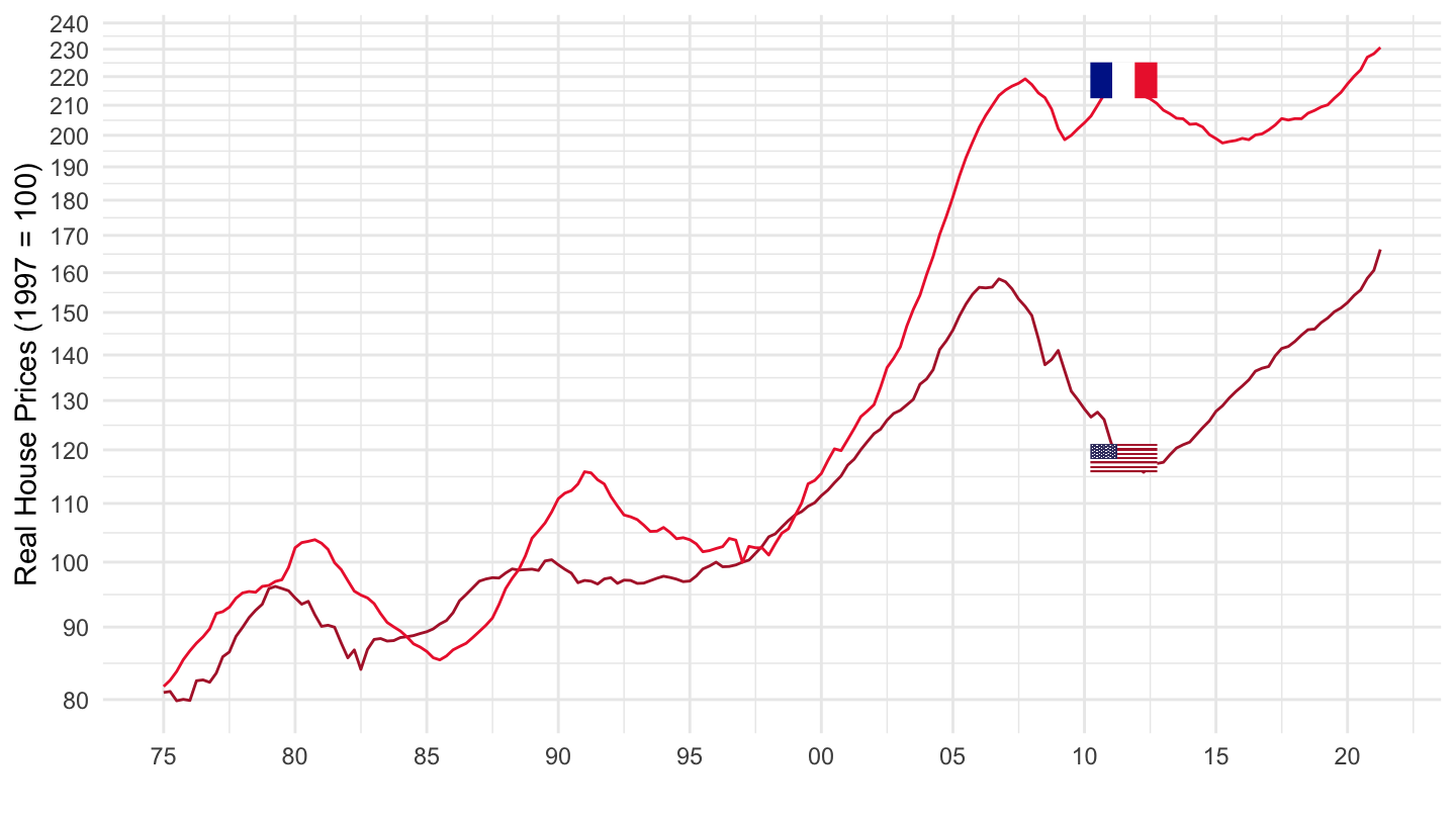
dallas_fed |>
  filter(countryname %in% c("Japan", "Korea", "Switzerland"),
         variable == "RHPI") |>
  add_flag_color("countryname") |>
  ggplot() + theme_minimal() + xlab("") + ylab("Real House Prices") +
  geom_line(aes(x = date, y = value, color = color)) +
  scale_color_identity() + add_3flags +
  scale_x_date(breaks = seq(1920, 2100, 5) |> paste0("-01-01") |> as.Date(),
               labels = date_format("%Y")) +
  scale_y_log10(breaks = c(seq(0, 500, 10), seq(10, 50, 10))) +
  theme(legend.position = c(0.25, 0.8),
        legend.title = element_blank())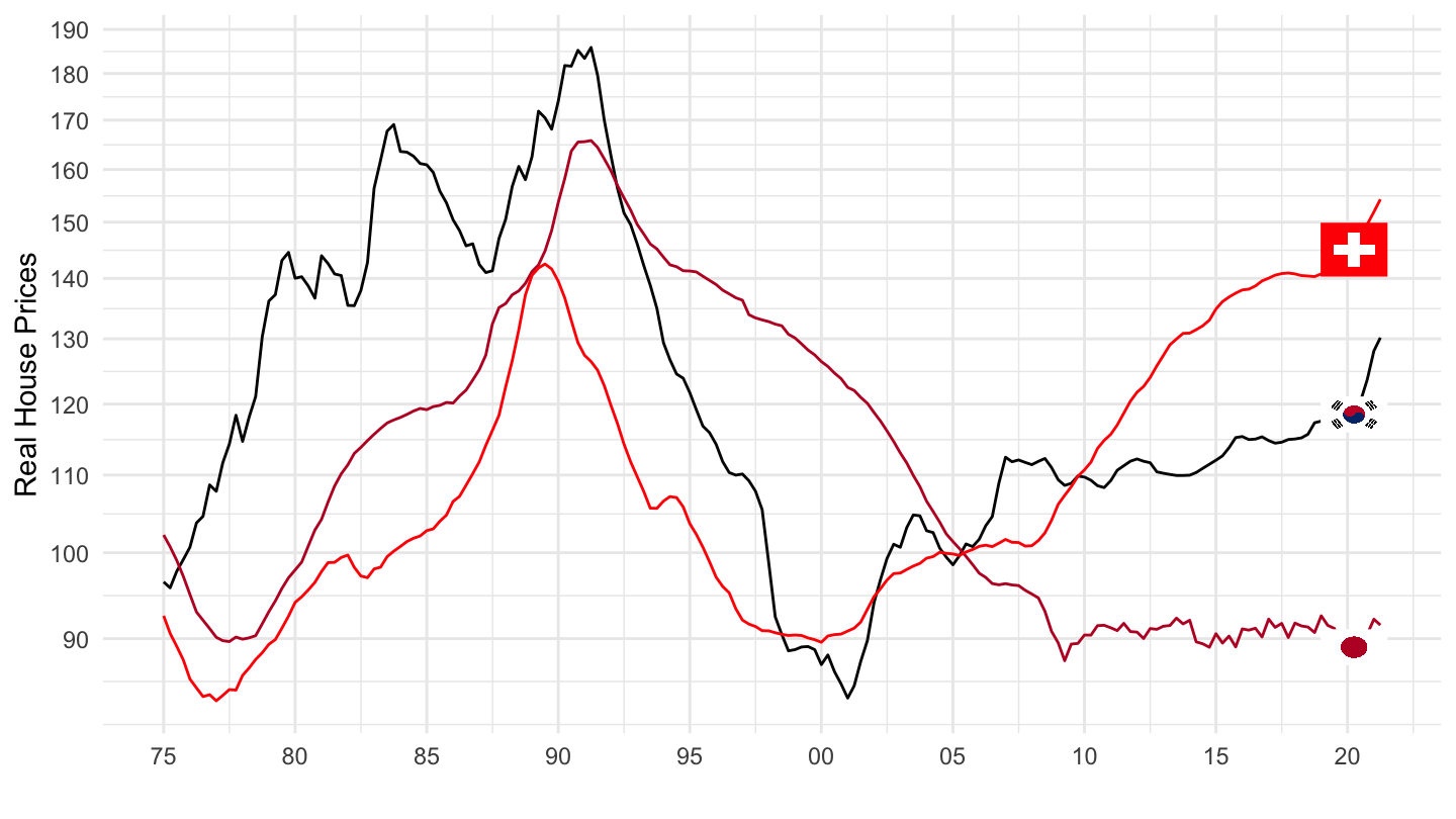
dallas_fed |>
  filter(countryname %in% c("Italy", "France", "United States"),
         variable == "RHPI") |>
  add_flag_color("countryname") |>
  ggplot() + theme_minimal() + xlab("") + ylab("Real House Prices") +
  geom_line(aes(x = date, y = value, color = color)) +
  scale_color_identity() + add_3flags +
  scale_x_date(breaks = seq(1920, 2100, 5) |> paste0("-01-01") |> as.Date(),
               labels = date_format("%Y")) +
  scale_y_log10(breaks = c(seq(0, 500, 10), seq(10, 50, 10))) +
  theme(legend.position = c(0.25, 0.8),
        legend.title = element_blank())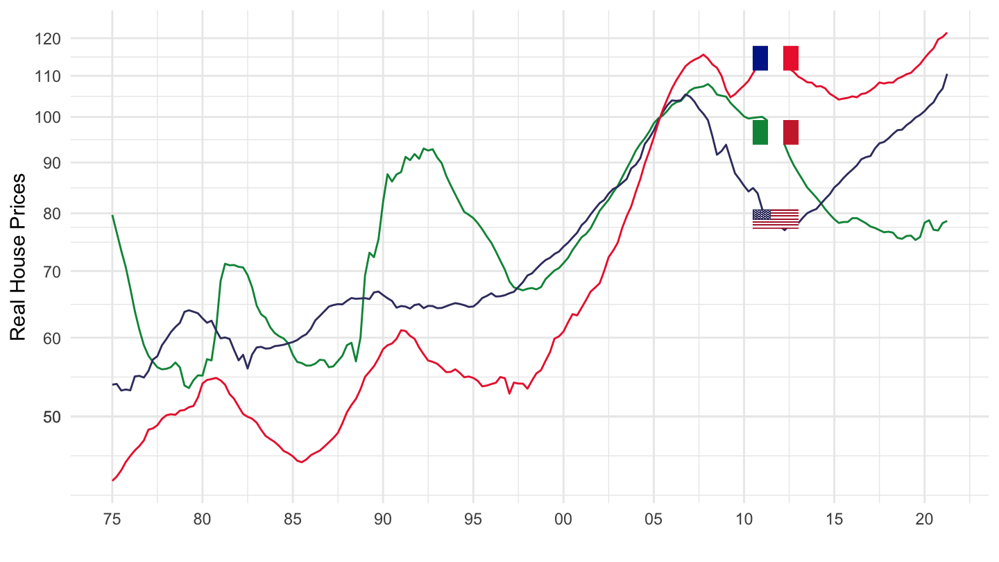
dallas_fed |>
  filter(countryname %in% c("Italy", "France", "United States", "Japan"),
         variable == "RHPI") |>
  add_flag_color("countryname") |>
  ggplot() + theme_minimal() + xlab("") + ylab("Real House Prices") +
  geom_line(aes(x = date, y = value, color = color)) +
  scale_color_identity() + add_4flags +
  scale_x_date(breaks = seq(1920, 2100, 5) |> paste0("-01-01") |> as.Date(),
               labels = date_format("%Y")) +
  scale_y_log10(breaks = c(seq(0, 500, 10), seq(10, 50, 10))) +
  theme(legend.position = c(0.25, 0.8),
        legend.title = element_blank())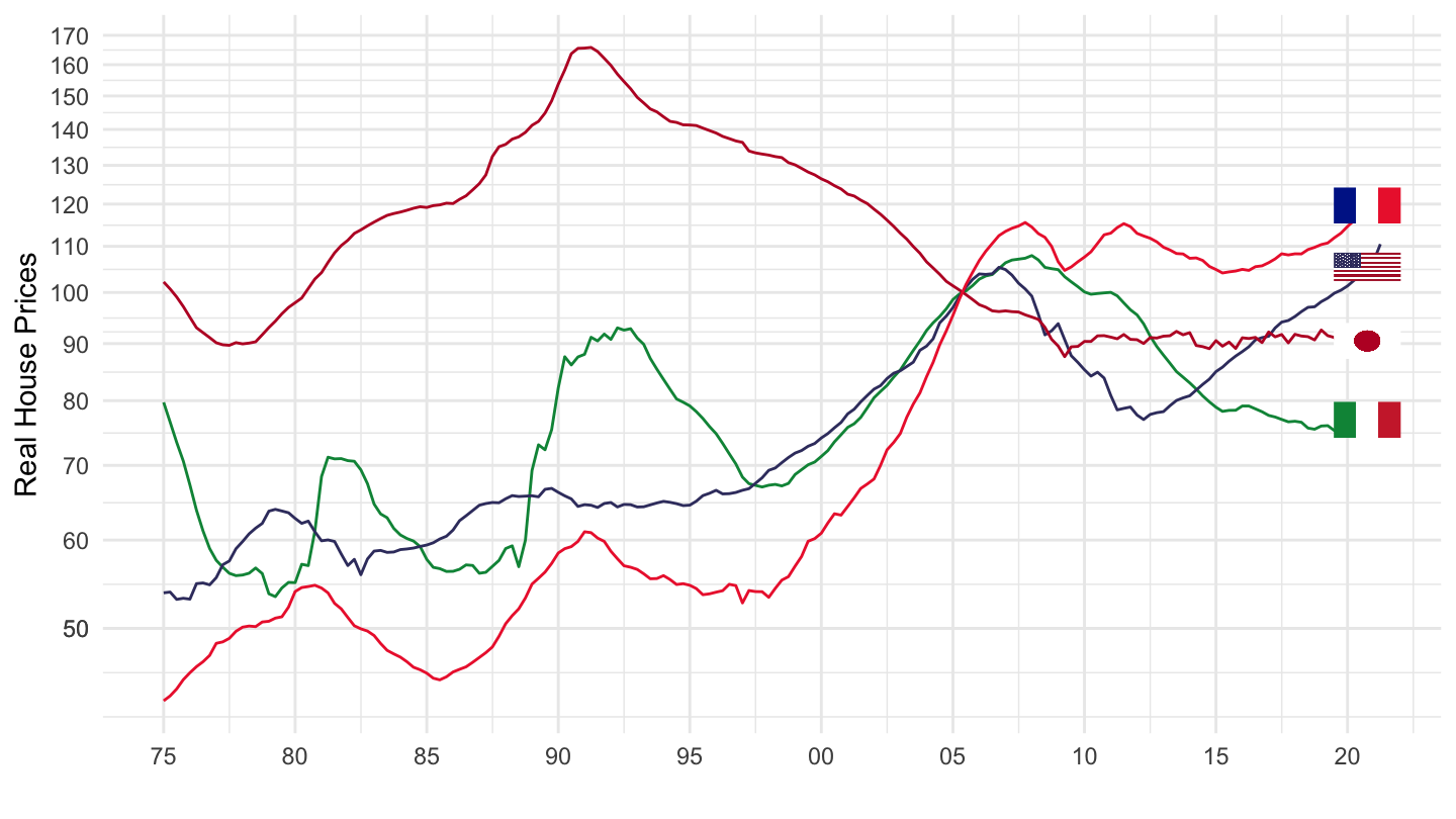
dallas_fed |>
  filter(countryname %in% c("Italy", "France", "United States", "Japan"),
         variable == "RPDI") |>
  add_flag_color("countryname") |>
  ggplot() + theme_minimal() + xlab("") + ylab("Real Price / Dividends Ratio") +
  geom_line(aes(x = date, y = value, color = color)) +
  scale_color_identity() + add_4flags +
  scale_x_date(breaks = seq(1920, 2100, 5) |> paste0("-01-01") |> as.Date(),
               labels = date_format("%Y")) +
  scale_y_log10(breaks = c(seq(0, 500, 10), seq(10, 50, 10))) +
  theme(legend.position = c(0.25, 0.8),
        legend.title = element_blank())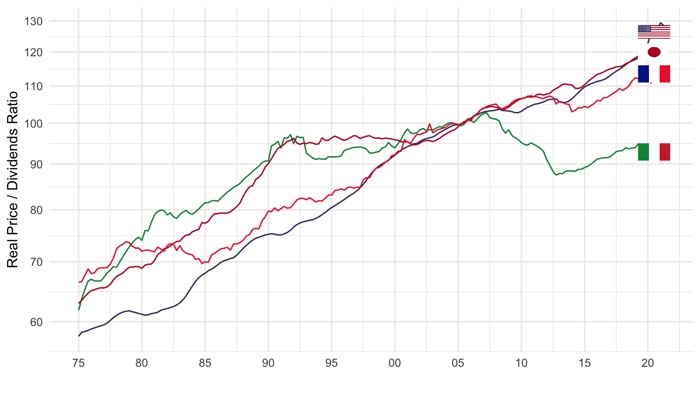
dallas_fed |>
  filter(countryname %in% c("Italy", "France", "United States", "Japan"),
         variable == "RPDI",
         date >= as.Date("1990-01-01")) |>
  add_flag_color("countryname") |>
  ggplot() + theme_minimal() + xlab("") + ylab("Real Price / Dividends Ratio") +
  geom_line(aes(x = date, y = value, color = color)) +
  scale_color_identity() + add_4flags +
  scale_x_date(breaks = seq(1920, 2100, 5) |> paste0("-01-01") |> as.Date(),
               labels = date_format("%Y")) +
  scale_y_log10(breaks = c(seq(0, 500, 10), seq(10, 50, 10))) +
  theme(legend.position = c(0.25, 0.8),
        legend.title = element_blank())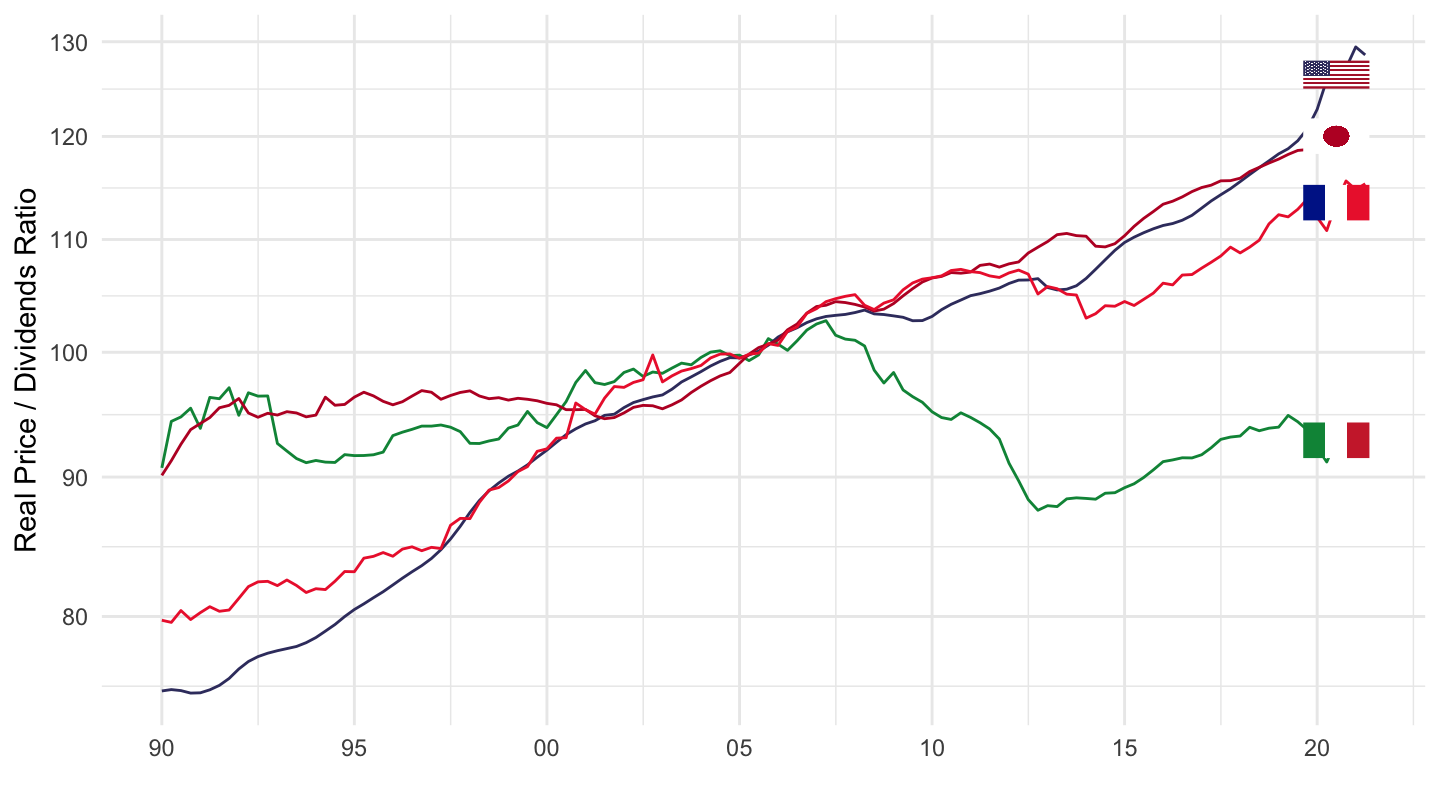
dallas_fed |>
  filter(countryname %in% c("Italy", "France", "United States", "Japan"),
         variable == "PDI") |>
  add_flag_color("countryname") |>
  ggplot() + theme_minimal() + xlab("") + ylab("Real Price / Dividends Ratio") +
  geom_line(aes(x = date, y = value, color = color)) +
  scale_color_identity() + add_4flags +
  scale_x_date(breaks = seq(1920, 2100, 5) |> paste0("-01-01") |> as.Date(),
               labels = date_format("%Y")) +
  scale_y_log10(breaks = c(seq(0, 500, 10), seq(10, 50, 10))) +
  theme(legend.position = c(0.25, 0.8),
        legend.title = element_blank())