Should Keynesian Economics Abandon the Phillips Curve?
monetary policy
inflation
unemployment
Phillips curve
[🌐 HTML Presentation] [🎞️ PDF Presentation] [📄 PDF Article]
In 1990, Larry Summers published an article critical of (New-)Keynesian orthodoxy entitled “Should Keynesian Economics Dispense with the Phillips Curve?”, in which he argued that (New-)Keynesianism displayed “many of the attributes that Thomas Kuhn has ascribed to dying scientific paradigms”. After listing the empirical and theoretical shortcomings of the Phillips curve, he compared (New-)Keynesian economics to Ptolemaic astronomy awaiting its Copernican revolution.
Yet, 30 years later, nothing has changed: although the Phillips curve has repeatedly disappointed—missing inflation in the United States in the late 1990s despite strong growth and unemployment below 4%, missing deflation during the 2007–2009 financial crisis and the European austerity period of 2011–2013—it remains at the core of New Keynesian macroeconomic models, particularly the dynamic stochastic general equilibrium (DSGE) models used in central banks and finance ministries around the world to design economic policy.
To understand this paradox, one must first revisit some key stages in the history of the Phillips curve, as well as the different views regarding the role that economic policy should consequently play in addressing unemployment. A new approach is then proposed and discussed, in which the Phillips curve is no longer a relationship between inflation and unemployment, but between the real exchange rate and unemployment: only the relative price of non-tradable goods to tradable goods, rather than prices themselves, is inversely related to unemployment. The implications of this empirical regularity for the conduct of economic policy are then examined.
A brief history of the Phillips curve, from full employment to structural unemployment
The history of the Phillips curve is complex and includes many episodes and turning points (Hoang-Ngoc 2007; Le Bihan 2009). At each of these stages, the understanding of the role of economic policy in addressing unemployment has evolved.
After the Second World War, Keynesian ideas triumphed, as military orders placed with the United States helped bring an end to the unemployment that had prevailed during the 1930s, as Keynes had anticipated. After 1945, it became clear to both economists and policymakers that economic policy, through active demand management, should aim at full employment. For example, the U.S. Employment Act of 1946 set the objective of “maximum employment.” The identification in 1958 by A.W. Phillips of a negative correlation between nominal wage inflation and unemployment in the United Kingdom over the period 1861–1913 gradually changed the landscape (Phillips 1958).
The “Phillips curve,” broadly understood as a relationship between inflation and unemployment, quickly became a standard relationship in macroeconomics through the work of Paul Samuelson and Robert Solow, two MIT professors, who popularized Phillips’s article, described a similar relationship for the United States in 1960, and progressively made this curve the core of the neoclassical synthesis (Samuelson and Solow 1960). The Phillips curve appeared to describe a process of gradual return to equilibrium (a tâtonnement process) in the labor market: when involuntary unemployment is high, wages fall, encouraging hiring. Conversely, when involuntary unemployment is low, wages rise, discouraging it. For proponents of the neoclassical synthesis, the Phillips curve thus provided evidence of “nominal rigidities,” demonstrating the inability of the economy to adjust to shocks in the short run through sufficiently rapid changes in wages and prices. Macroeconomics is Keynesian in the short run (policies supporting demand can help reduce unemployment) and classical in the long run (only supply determines it). The trade-off between unemployment and inflation described by the Phillips curve forces policymakers to choose, in the short run, a combination of unemployment and inflation, under the constraint that low unemployment comes at the cost of high inflation. The Phillips curve thus constituted a first breach in the fight against unemployment: full employment as defined by the Employment Act became unattainable, as achieving it would require tolerating very high inflation. Yann Giraud describes MIT Keynesianism as a position “midstream,” between full-employment Keynesianism and the neoclassical view according to which involuntary unemployment does not exist (Giraud 2014).
A second breach in the fight against unemployment emerged at the end of the 1960s with Edmund Phelps and Milton Friedman, both future Nobel laureates in economics. For them, short-term stabilization policies could reduce unemployment only at the cost not merely of higher inflation, but of accelerating inflation. The Phillips curve thus became a relationship not between inflation and unemployment, but between the change in inflation and the gap between the unemployment rate and the structural unemployment rate—the latter being the level below which unemployment should not fall without triggering accelerating inflation. For Milton Friedman, this implied that expansionary policies would entail ever-increasing inflation, a much less favorable trade-off for Keynesian policies. Conversely, unemployment only leads to a deceleration of inflation and is not necessarily associated with lower inflation initially, implying that unemployment and inflation can coexist in the short run. The stagflation of the 1970s—a combination of high inflation and high unemployment—seemed to confirm this view. Olivier Blanchard and Daniel Cohen, in their macroeconomics textbook (Blanchard and Cohen 2020), conclude: “Friedman could not have put it better: a few years later, the original Phillips curve began to disappear, exactly as Friedman had predicted.”
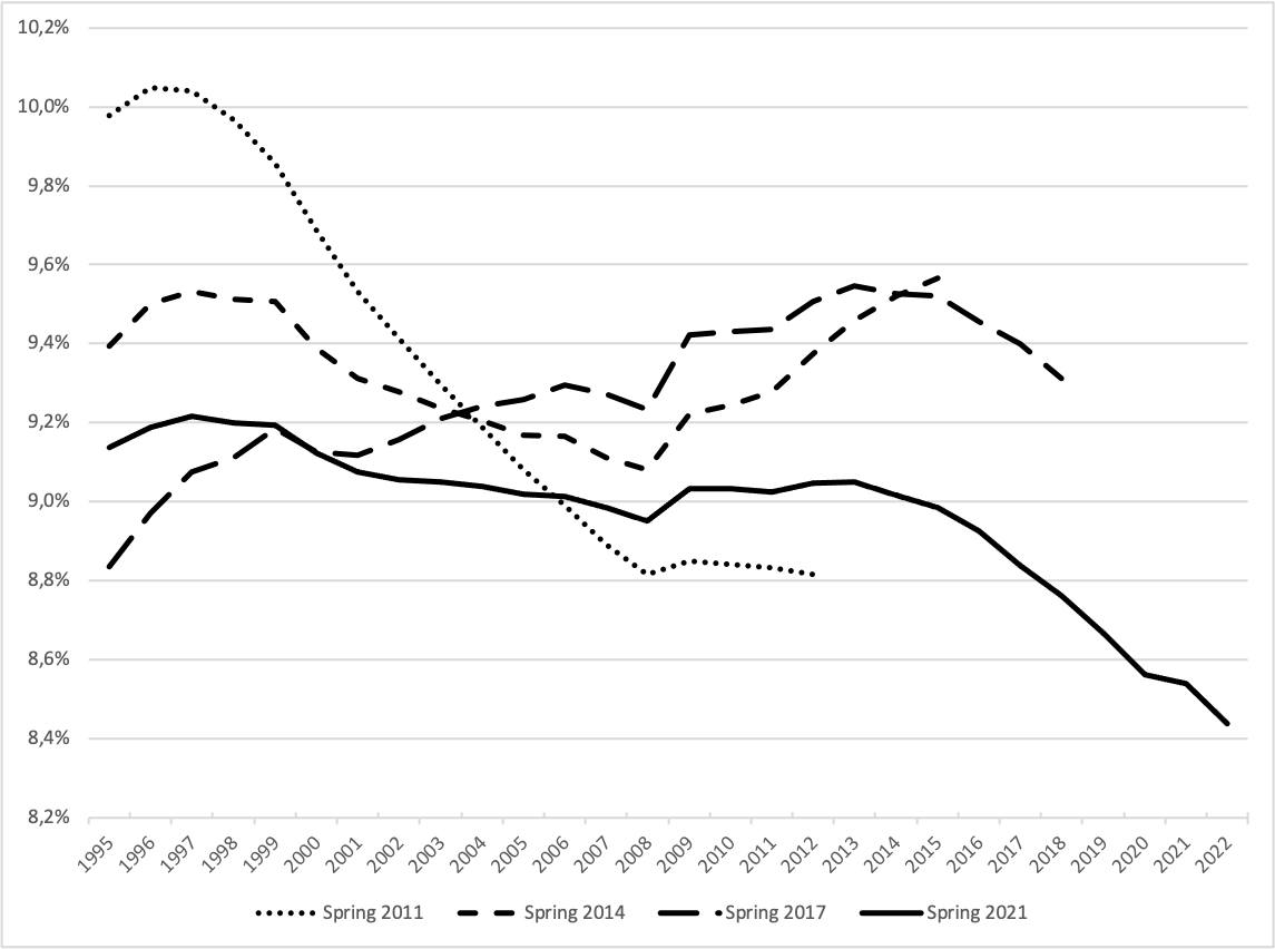
The analysis of Phelps and Friedman has two major implications relative to the original Phillips curve. First, it implies the existence of a structural unemployment rate that does not accelerate inflation—the Non-Accelerating Inflation Rate of Unemployment (NAIRU). Second, it requires incorporating inflation expectations into what is known as the “augmented” Phillips curve. These contributions are taken up by New Keynesian economists, who differ from Milton Friedman only in that they believe stabilization policies can help bring unemployment back to its structural level, rather than relying solely on market forces. The NAIRU, as estimated by institutions such as the OECD, the IMF, the European Commission, and the Banque de France, is generally assessed at a high level—around 9% in France. This leads to diagnosing a risk of overheating—that is, accelerating inflation—as soon as unemployment falls below this level. Yet these estimates are frequently revised, as shown in Figure 1: for example, for 2018, the structural unemployment rate was estimated at 9.3% in spring 2017, but at 8.8% four years later, suggesting that the overheating risk was lower than initially thought. From a policy perspective, this also leads to a greater focus on the structural and microeconomic causes of unemployment and, consequently, on labor market flexibility policies, which, within this paradigm, are seen as the only way to reduce structural unemployment. However, this revised version of the Phillips curve was quickly contradicted by the facts: in the late 1990s, for example, the “dot-com bubble” brought unemployment below 4% in the United States—well below the NAIRU—without any increase in inflation; similarly, in early 2020 before the COVID-19 crisis, Donald Trump’s expansionary policies reduced unemployment to 3.5%, again without any rise in inflation. This raises the question, in hindsight, of whether the stagflation of the 1970s provided a sufficient basis for adopting the theory of structural unemployment.
The Phillips curve of the real exchange rate
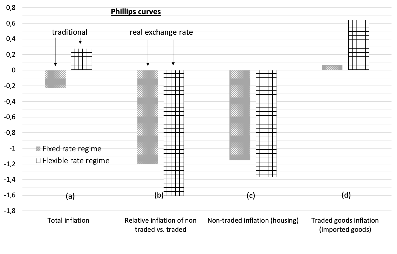
What has been overlooked in particular is that the disappearance of the Phillips curve in the 1970s in the United States coincided with the end, in 1971, of the Bretton Woods system, under which currencies were pegged to the dollar, itself fixed in terms of gold. More generally, with hindsight, it appears that Phillips curves linking inflation and unemployment have always been identified in countries operating under fixed exchange rate regimes: in Great Britain between 1861 and 1913 (then under the gold standard), which inspired Phillips’s original work; between U.S. states, between regions within a country, between euro area countries, or between countries sharing the same currency (Geerolf 2018). This holds more generally, as shown in Figure 2(a) using data from Ilzetzki et al. (2019): under fixed exchange rates, a 1% increase in the unemployment rate is associated with a 0.2% decrease in inflation. But under flexible exchange rate regimes, on average, a 1% increase in unemployment is associated with an increase in inflation of nearly 0.3%.
If, however, one relates the unemployment rate not to inflation but to changes in the real exchange rate—that is, the relative inflation of non-tradable goods compared to tradable goods—one observes a negative relationship between unemployment and real exchange rate appreciation regardless of the exchange rate regime (Figure 2(b)). This does not invalidate the traditional Phillips curve under fixed exchange rates, insofar as inflation and real exchange rate appreciation coincide, but this is not the case under flexible exchange rates. Decomposing total inflation into its components (non-tradable and tradable goods) helps explain why.
Under both fixed and flexible exchange rate regimes, a decline in unemployment following an increase in demand is accompanied by upward pressure on demand for non-tradable goods, whose supply is limited, leading to higher prices—this is particularly the case for housing prices (Figure 2(c)). The relationship between unemployment and inflation of non-tradable goods is therefore negative under both fixed and flexible regimes.
For tradable goods, depending on whether countries operate under fixed or flexible exchange rate regimes, the relationship between unemployment and inflation (of tradable goods) is either zero (under fixed exchange rates)—since the price of these goods is determined on global markets and the exchange rate does not vary, there is no reason to observe a systematic relationship with unemployment—or positive (under flexible exchange rates), as the nominal exchange rate appreciates when unemployment falls, which pushes down the price of tradable goods in domestic currency (Figure 2(d)). This nominal appreciation results from central bank actions to contain inflation: as seen earlier, a decline in unemployment is associated with rising inflation in non-tradable goods, which, to be countered, requires an increase in policy interest rates, leading—under flexible exchange rates—to an appreciation of the currency.
To summarize, the relationship between unemployment and inflation of tradable goods is either zero under fixed exchange rates or positive under flexible exchange rates; the relationship between unemployment and inflation of non-tradable goods is negative regardless of the exchange rate regime. The results for total inflation (a), corresponding to the traditional Phillips curve, are obtained by calculating the weighted average of the effects on inflation of non-tradable goods (c) and tradable goods (d). Those for relative inflation (b), corresponding to the real exchange rate Phillips curve, are obtained by subtracting the effect on tradable goods inflation (d) from that on non-tradable goods inflation (c).
The real exchange rate Phillips curve accounts for many observations that contradict the traditional Phillips curve—again, for countries under flexible exchange rate regimes—while also explaining the cases in which the Phillips curve does apply—namely under fixed exchange rates. For example, the real exchange rate Phillips curve is consistent with episodes of stagflation observed in Latin American countries following exchange rate crises. In December 2001, Argentina devalued the peso, which had been pegged to the dollar since 1990 (1 dollar = 1 peso), by more than 60% (1 dollar = 3 pesos), while unemployment stood at around 15%. This immediately put an end to the deflation that had accompanied rising unemployment since 1996: inflation rose to 26% in 2002 and then to 13% in 2003. What we observe is indeed a depreciation of the real exchange rate, as the nominal devaluation exceeded the resulting increase in inflation. The dichotomy between fixed and flexible exchange rates also explains why Phillips curves can be observed across countries or regions within a country sharing a common currency, but not for economies under flexible exchange rates. For example, during the European austerity period of 2010–2013, the euro area—whose exchange rate is flexible—did not experience deflation: inflation even exceeded 2% in 2011 and 2012, prompting the ECB to raise interest rates. However, the European countries most affected by fiscal austerity did experience disinflation or even deflation—such as Greece at the end of 2012—because their exchange rate is effectively fixed. Finally, further support for the real exchange rate Phillips curve comes from the fact that, under flexible exchange rates, a decline in unemployment is associated not with inflation but with an appreciation of the nominal exchange rate, which lowers import prices and explains, for example, the absence of inflationary pressures in the United States in the late 1990s: between 1995 and 1999, the decline in unemployment from 5.6% to 4.3% was accompanied not by rising but by falling inflation—from 2.3% to 1.5%—along with an appreciation of the dollar of about 30% against other currencies and a 15% decline in import prices.
One of the appealing features of the traditional Phillips curve, which likely contributed to its success, is its intuitive nature: a decline in unemployment would increase workers’ bargaining power, allowing them to demand higher (nominal) wages. In reality, this intuition is based on a flawed argument. If the Phillips curve is interpreted as an equilibrium between supply and demand in the labor market, then it determines the real wage rather than the nominal wage (since, according to general equilibrium theory, the interaction of supply and demand determines only relative prices of goods and factors). Thus, a decline in unemployment should lead to an increase in real wages, but there is no theoretical reason why this mechanism should determine nominal wage inflation. James Tobin himself noted that the Phillips curve was “an empirical observation in search of a theoretical explanation” (Tobin 1972).
By contrast, the real exchange rate Phillips curve admits several theoretical justifications. To see this, one should not start from a decline in unemployment, but from its underlying causes: an increase in aggregate demand or a productivity increase in the export sector (where most productivity gains are observed in practice). In the case of higher aggregate demand, firms’ order books fill up, prompting them to hire and reducing unemployment. This also leads to an increase in the price of domestically produced goods—that is, an increase in the price of non-tradable goods relative to tradable goods (hence an appreciation of the real exchange rate)—since non-tradable goods cannot be imported and their supply is less elastic. An increase in productivity in the export sector, for its part, allows firms to gain market share abroad because export prices can decline. The resulting increase in exports leads to more hiring in the export sector and higher real wages, without increasing prices due to productivity gains. In contrast, in the non-tradable sector—which competes with the tradable sector for labor but does not benefit from the same productivity gains—prices increase. In both cases, lower unemployment is associated with a higher real exchange rate.
A competitiveness problem
The “revisited” Phillips curve thus shows that the trade-off policymakers face is not between inflation and unemployment, but between competitiveness losses and unemployment. Stimulating demand to reduce unemployment leads to an appreciation of the real exchange rate, which undermines competitiveness and, with it, the trade balance. This results in a rapid decline in the share of industry in value added (accelerated deindustrialization), which may lead to excessive development of low-productivity, sheltered sectors such as construction and services. This also limits the ability to generate trade surpluses in the future and slows productivity growth, which is weaker in sheltered services than in industry (and tradable services). As early as the 1970s, these detrimental effects of demand stimulus on competitiveness concerned Richard Nixon, who worried that the United States might end up producing only “toilet paper and toothpaste.” Juanita Kreps, Secretary of Commerce under Jimmy Carter, even chose in 1979 to resign from her academic position after her government experience, no longer knowing “what to teach.”
This dilemma between competitiveness and stimulus is, however, rejected by New Keynesian economists. According to Paul Krugman in Pop Internationalism (Krugman 1998): “Employment growth in the United States depends not on its ability to sell on world markets or compete with imports, but on decisions by the Federal Reserve to counter inflation.” The traditional Phillips curve thus leads to a conclusion opposite to that of the real exchange rate Phillips curve. In the traditional view, there is no need to worry about competitiveness in general, or industrial employment in particular, since increasing industrial employment would necessarily generate inflationary pressures, all else equal. The real exchange rate Phillips curve, by contrast, leads to a partial rehabilitation of mercantilist ideas and of the importance of external balances, consistent with Keynes’s analysis in Chapter 24 of The General Theory, where he supported the traditional view of practitioners against that of classical economists: “For about two hundred years, neither economists nor businessmen ever doubted that a favorable balance of trade was a serious advantage for a country and an unfavorable balance a grave danger.”
Thus, the policy implications derived from the real exchange rate Phillips curve differ radically from those of the New Keynesian open-economy model, the Mundell–Fleming model. In the latter, competitiveness problems arise only under fixed exchange rates, since under flexible exchange rates the exchange rate adjusts automatically. By contrast, the real exchange rate Phillips curve implies that potential competitiveness problems exist regardless of the exchange rate regime. This is illustrated, for example, by the United States in the early 1980s, whose industrial sector was severely damaged by the appreciation of the dollar (itself resulting from the increase in interest rates decided by Paul Volcker to combat inflation).
Moreover, the real exchange rate Phillips curve implies that trade imbalances cannot be reduced to insufficient adjustment of prices and wages. As a result, “nominal convergence” policies advocated in the euro area—consisting of reducing nominal wages in deficit countries—are far less effective than predicted by the Mundell–Fleming model (Geerolf and Grjebine 2020). In addition, trade imbalances are not temporary, as evidenced by the persistence of Germany’s trade surplus at around 7% of GDP for the past 20 years. J.M. Keynes in The General Theory explicitly warned against the idea that unemployment results from excessively high wages, although, as noted by De Vroey (2016) in his history of macroeconomics, one may question whether he fully completed the theoretical refoundation needed to support this claim.
Some concrete implications
The real exchange rate Phillips curve also has practical implications for thinking about macroeconomic policy. First, it helps put into perspective fears that Joe Biden’s stimulus plan would trigger an “inflationary spiral,” that is, ever-accelerating inflation as in the 1960s–1970s. The U.S. experience of the 1960s—during which declining unemployment was associated with rising inflation between 1960 and 1969—is often cited in support of this concern (Blanchard 2021). The real exchange rate Phillips curve shows that this comparison is not relevant for assessing current developments: at the time, the United States was operating under the Bretton Woods system, in which inflation and the real exchange rate coincided, whereas today it operates under flexible exchange rates. In particular, the real exchange rate Phillips curve suggests that overheating risks are concentrated in the housing market and that inflationary pressures could be mitigated by an appreciation of the dollar.
This also calls into question the relevance of inflation-targeting policies adopted by most central banks since the 1990s, or at least whether they are sufficient to both stabilize inflation and achieve satisfactory employment levels. According to New Keynesian economists, under the augmented Phillips curve, stabilizing inflation also stabilizes economic activity at its potential level and unemployment at its structural level. A corollary of inflation targeting is monetary dominance—the idea that monetary policy should take precedence in macroeconomic stabilization, while fiscal policy should be limited to allowing automatic stabilizers to operate (such as unemployment benefits). However, in a context where stable inflation can coexist with high unemployment (if the nominal exchange rate depreciates), stabilizing inflation is no longer sufficient: fiscal policy must be used discretionarily to ensure that unemployment remains at an acceptable level. In the 1990s, questioning monetary dominance would have led a Keynesian economist to be labeled a “vulgar” Keynesian (Krugman 1997). Today, however, questioning the interaction between monetary and fiscal policy has become more widely accepted, as illustrated by Fabio Panetta’s speech on June 30, 2021, in which the ECB Executive Board member stated that “the experience accumulated since the 2007–09 financial crisis shows that situations in which monetary and fiscal policies must work together are not exceptional.”
The questioning of inflation targeting has direct implications for current debates surrounding central banks’ strategic reviews. In the case of the Federal Reserve, monetary policy already has a dual mandate of price stability and maximum employment. As part of its recent policy review, the Fed has strengthened the weight given to its employment objective relative to inflation. In particular, the employment objective has become asymmetric: monetary policy decisions will no longer be based on deviations of employment from its maximum level, but on shortfalls relative to that level—subtly indicating that “employment can be at or above real-time estimates of its maximum level without causing concern” and reflecting the Fed’s view that “a robust labor market can be sustained without triggering a surge in inflation.” This is a barely veiled expression of the institution’s skepticism toward the Phillips curve, which Jerome Powell, the Fed Chair, described in June 2021 as part of “our old models,” and which Daniel Tarullo, former Board member, considered a “non-operational theory” (Tarullo 2017). This skepticism is not limited to the institution itself, as illustrated by Alexandria Ocasio-Cortez’s intervention in 2019, when she questioned Jerome Powell during a congressional hearing about the validity of the Phillips curve and the policy mistakes made in its name—an intervention praised by Larry Kudlow, then head of Donald Trump’s National Economic Council.
At the European Central Bank, such reassessments of the Phillips curve remain more limited. However, the proposal, as part of the strategic review announced on July 8, 2021, to give greater weight to housing prices in the consumer price index—by including imputed rents for owner-occupiers—can be justified by the real exchange rate Phillips curve, according to which such prices are a better indicator of demand pressures than the general price level. The Reserve Bank of New Zealand, which pioneered inflation targeting in December 1989, has in fact explicitly incorporated housing prices into its monetary policy objectives since March 2021. Similar reflections are underway at the Fed, as the feared overheating once again appears primarily in housing prices.
In conclusion, it is high time that New Keynesian economics in particular, and macroeconomics more broadly, dispense with the Phillips curve. Empirical analysis shows that the traditional Phillips curve is not (and has never been) observed under flexible exchange rates. The implications are numerous, particularly for the design of economic policy, as this paper has sought to demonstrate. More generally, the Phillips curve illustrates the need for greater reliance on empirical analysis to understand macroeconomic phenomena, and less reliance on a priori theoretical models disconnected from reality or based on partial empirical evidence. The credibility of economists and of economics as a “science” depends on it.
References
Blanchard, Olivier. 2021. “In Defense of Concerns over the $1.9 Trillion Relief Plan PIIE.” In Peterson Institute for International Economics Realtime Economic Issues Watch. https://www.piie.com/blogs/realtime-economics/defense-concerns-over-19-trillion-relief-plan.
Blanchard, Olivier, and Daniel Cohen. 2020. Macroéconomie, 8ème Édition. Pearson. HAL. https://ideas.repec.org/p/hal/pseptp/halshs-02921644.html.
De Vroey, Michel. 2016. A History of Macroeconomics from Keynes to Lucas and Beyond. Cambridge University Press.
Geerolf, François. 2018. The Phillips Curve: A Relation Between Real Exchange Rate Growth and Unemployment. UCLA Working Paper. https://fgeerolf.com/phillips.pdf.
Geerolf, François, and Thomas Grjebine. 2020. “Rééquilibrage de La Zone Euro : Plus Facile Avec Le Bon Diagnostic !” La Lettre Du CEPII, no. 411 (October).
Giraud, Yann. 2014. “Negotiating the ‘Middle-of-the-Road’ Position: Paul Samuelson, Mit, and the Politics of Textbook Writing, 1945-55.” History of Political Economy 46 (December): 134–52. https://doi.org/10.1215/00182702-2716145.
Hoang-Ngoc, Liêm. 2007. Le Fabuleux Destin de La Courbe de Phillips : Les Théories de l’inflation Et Du Chômage Après Keynes. Presses Universitaires du Septentrion. https://www.septentrion.com/fr/book/?GCOI=27574100273170.
Ilzetzki, Ethan, Carmen M. Reinhart, and Kenneth S. Rogoff. 2019. “Exchange Arrangements Entering the Twenty-First Century: Which Anchor Will Hold?” The Quarterly Journal of Economics 134 (2): 599–646. https://doi.org/10.1093/qje/qjy033.
Krugman, Paul. 1997. “Vulgar Keynesians. A Penny Spent Is Not a Penny Earned ?” Slate - Dismal Scientist, February. https://web.mit.edu/krugman/www/vulgar.html.
Krugman, Paul. 1998. La Mondialisation n’est Pas Coupable. Vertus Et Limites Du Libre-Échange. La Découverte. https://www.decitre.fr/livres/la-mondialisation-n-est-pas-coupable-9782707131133.html.
Le Bihan, Hervé. 2009. “1958-2008, Avatars Et Enjeux de La Courbe de Phillips.” Revue de l’OFCE n° 111 (4): 81–101. https://www.cairn.info/revue-de-l-ofce-2009-4-page-81.htm.
Phillips, A. W. 1958. “The Relation Between Unemployment and the Rate of Change of Money Wage Rates in the United Kingdom, 1861-1957.” Economica 25 (100): 283–99. https://doi.org/10.1111/j.1468-0335.1958.tb00003.x.
Samuelson, Paul A., and Robert M. Solow. 1960. “Analytical Aspects of Anti-Inflation Policy.” The American Economic Review 50 (2): 177–94. http://www.jstor.org/stable/1815021.
Tarullo, Daniel K. 2017. Monetary Policy Without a Working Theory of Inflation. Hutchins Center Working Paper. https://www.brookings.edu/research/monetary-policy-without-a-working-theory-of-inflation/.
Tobin, James. 1972. “Inflation and Unemployment.” The American Economic Review 62 (1/2): 1–18. https://www.jstor.org/stable/1821468.