
Last observation: 7 oct. 2026 (N = 2859)
First observation: 2 janv. 1980 (N = 181)
Last data update: 07 oct. 2026, 23:29
Last compile: 07 oct. 2026, 23:36
Cours quotidiens Yahoo Finance de 3 073 sociétés du catalogue investing.com américain (stocks_USA_var), depuis 1980. Le ticker Yahoo est retrouvé par ISIN (adjusted_map.parquet) ; l’univers inclut quelques cotations étrangères (Francfort, Toronto…) qu’on écarte dans les statistiques d’ensemble (NYSE, NASDAQ, NYSE MKT).
Close = cours de clôture corrigé des splits seulement ; Adjusted = cours corrigé des splits et des dividendes (dividendes réinvestis), donc Adjusted mesure le rendement total. Le rapport Adjusted / Close à une date donnée est le facteur cumulé des dividendes versés après cette date.
adj |> mutate(year = year(Date)) |> group_by(year) |>
  summarise(Titres = n_distinct(ticker), Lignes = n(), .groups = "drop") |>
  filter(year %% 5 == 0 | year == max(year)) |>
print_table_conditional()| year | Titres | Lignes |
|---|---|---|
| 1980 | 410 | 88949 |
| 1985 | 540 | 132568 |
| 1990 | 715 | 177968 |
| 1995 | 1100 | 266541 |
| 2000 | 1554 | 383050 |
| 2005 | 1835 | 453889 |
| 2010 | 2289 | 563992 |
| 2015 | 2688 | 666730 |
| 2020 | 2952 | 745390 |
| 2025 | 3020 | 753814 |
| 2026 | 3073 | 580871 |
adj |> mutate(year = year(Date)) |> group_by(year) |> summarise(n = n_distinct(ticker)) |>
  ggplot(aes(year, n)) + geom_line() + theme_minimal() + xlab("") + ylab("Nombre de titres")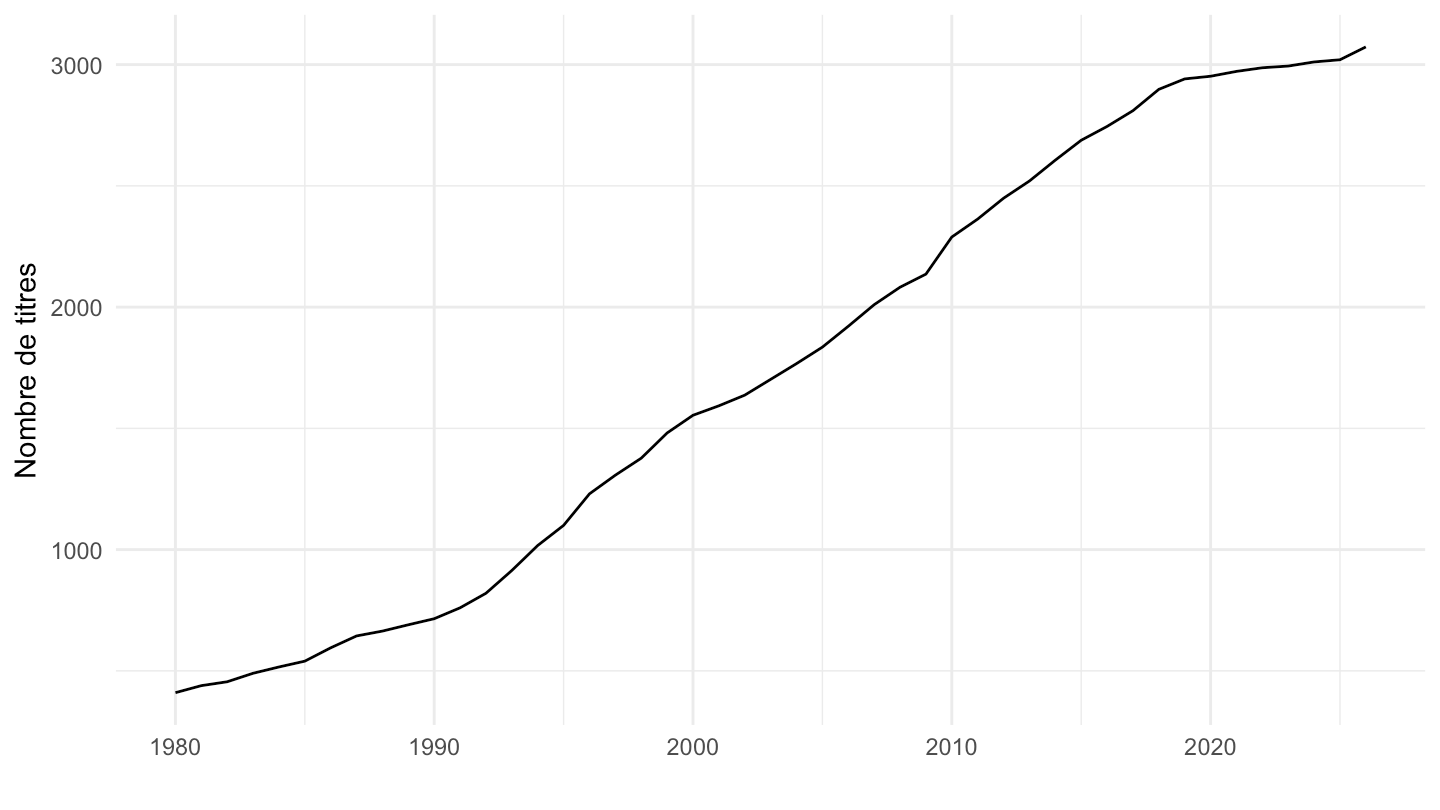
ex <- c("KO", "JNJ", "XOM", "PG", "MSFT", "AAPL", "T", "IBM")
d <- adj |> filter(ticker %in% ex, Date >= as.Date("1995-01-01"), Adjusted > 0, Close > 0) |>
  group_by(ticker) |> arrange(Date) |>
  mutate(`Cours (hors dividendes)` = 100 * Close / first(Close),
         `Cours ajusté (dividendes réinvestis)` = 100 * Adjusted / first(Adjusted)) |> ungroup() |>
  pivot_longer(c(`Cours (hors dividendes)`, `Cours ajusté (dividendes réinvestis)`), names_to = "serie", values_to = "y")
ggplot(d, aes(Date, y, color = serie)) + geom_line(linewidth = 0.5) + facet_wrap(~ticker, scales = "free_y") +
  scale_y_log10() + theme_minimal() + xlab("") + ylab("Base 100 (échelle log)") +
  theme(legend.position = "bottom", legend.title = element_blank())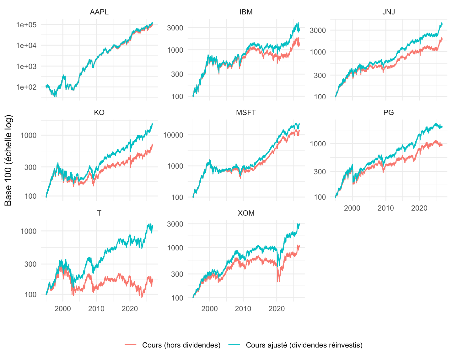
adj |> filter(ticker %in% ex, Adjusted > 0, Close > 0) |> group_by(ticker) |> arrange(Date) |>
  summarise(Début = first(Date), `Années` = as.numeric(last(Date) - first(Date)) / 365.25,
            `Cours seul (%/an)` = 100 * ((last(Close) / first(Close))^(1 / `Années`) - 1),
            `Avec dividendes (%/an)` = 100 * ((last(Adjusted) / first(Adjusted))^(1 / `Années`) - 1),
            `Ecart = dividendes (pp/an)` = `Avec dividendes (%/an)` - `Cours seul (%/an)`, .groups = "drop") |>
mutate(across(where(is.numeric), \(x) round(x, 2))) |> print_table_conditional()| ticker | Début | Années | Cours seul (%/an) | Avec dividendes (%/an) | Ecart = dividendes (pp/an) |
|---|---|---|---|---|---|
| AAPL | 1980-12-12 | 45.82 | 18.75 | 19.44 | 0.70 |
| IBM | 1980-01-02 | 46.76 | 5.93 | 8.97 | 3.05 |
| JNJ | 1980-01-02 | 46.76 | 11.49 | 14.19 | 2.70 |
| KO | 1980-01-02 | 46.76 | 10.82 | 14.02 | 3.20 |
| MSFT | 1986-03-13 | 40.57 | 23.62 | 25.15 | 1.53 |
| PG | 1980-01-02 | 46.76 | 9.29 | 12.42 | 3.13 |
| T | 1983-11-21 | 42.88 | 4.39 | 11.27 | 6.88 |
| XOM | 1980-01-02 | 46.76 | 8.67 | 13.33 | 4.67 |
Pour chaque titre avec au moins 10 ans d’historique : écart entre le rendement annualisé avec et sans dividendes (proxy du rendement de dividende moyen réinvesti).
gap <- adj |> inner_join(adj_map |> filter(exchange %in% c("NASDAQ", "NYSE", "NYSE MKT")) |> select(ticker), by = "ticker") |>
  filter(Adjusted > 0, Close > 0) |> group_by(ticker) |> arrange(Date) |>
  summarise(yrs = as.numeric(last(Date) - first(Date)) / 365.25,
            cagr_p = (last(Close) / first(Close))^(1 / yrs) - 1,
            cagr_a = (last(Adjusted) / first(Adjusted))^(1 / yrs) - 1, .groups = "drop") |>
  filter(yrs >= 10, is.finite(cagr_p), is.finite(cagr_a)) |>
  mutate(gap = 100 * (cagr_a - cagr_p))
gap |> summarise(Titres = n(), `Cours seul médian (%/an)` = 100 * median(cagr_p),
                 `Avec dividendes médian (%/an)` = 100 * median(cagr_a),
                 `Ecart médian (pp/an)` = median(gap), `Ecart moyen (pp/an)` = mean(gap),
                 `Part sans dividende (écart < 0,05)` = mean(gap < 0.05)) |>
mutate(across(where(is.numeric), \(x) round(x, 2))) |> print_table_conditional()| Titres | Cours seul médian (%/an) | Avec dividendes médian (%/an) | Ecart médian (pp/an) | Ecart moyen (pp/an) | Part sans dividende (écart < 0,05) |
|---|---|---|---|---|---|
| 2146 | 5.91 | 8.35 | 1.29 | 1.98 | 0.27 |
ggplot(gap |> filter(gap < 15), aes(gap)) + geom_histogram(bins = 60, fill = viridis::viridis(3)[1]) +
  theme_minimal() + xlab("Ecart de rendement annualisé, avec - sans dividendes (pp)") + ylab("Titres")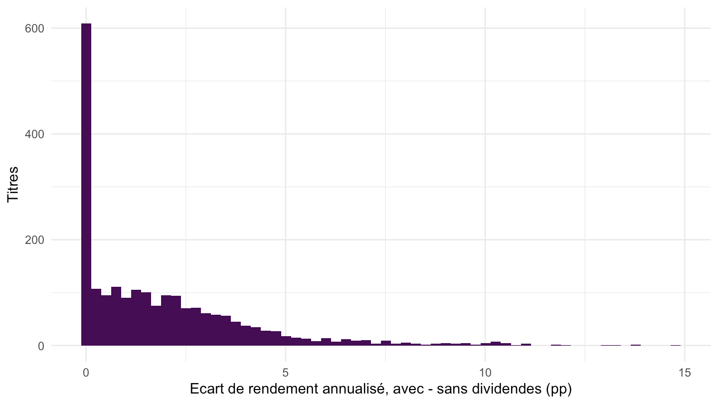
Moyenne simple des rendements mensuels des titres disponibles (au moins 20 titres), avec et sans dividendes. Attention au biais de survie : seuls les titres encore cotés figurent dans la base.
keep <- adj_map |> filter(exchange %in% c("NASDAQ", "NYSE", "NYSE MKT")) |> pull(ticker)
dt <- as.data.table(adj)[ticker %in% keep & Adjusted > 0 & Close > 0]
dt[, month := as.Date(format(Date, "%Y-%m-01"))]
mo <- dt[order(Date), .(Close = last(Close), Adjusted = last(Adjusted)), by = .(ticker, month)]
setorder(mo, ticker, month)
mo[, `:=`(rp = Close / shift(Close) - 1, ra = Adjusted / shift(Adjusted) - 1,
          gap = as.numeric(month - shift(month))), by = ticker]
ew <- mo[!is.na(rp) & gap <= 31 & abs(rp) < 1 & abs(ra) < 1,
         .(n = .N, Prix = mean(rp), `Rendement total` = mean(ra)), by = month][n >= 20][order(month)]
ew_l <- ew |> pivot_longer(c(Prix, `Rendement total`), names_to = "serie", values_to = "r") |>
  group_by(serie) |> arrange(month) |> mutate(y = 100 * cumprod(1 + r)) |> ungroup()
ggplot(ew_l, aes(month, y, color = serie)) + geom_line() + scale_y_log10() + theme_minimal() +
  xlab("") + ylab("Base 100 (échelle log)") + theme(legend.position = c(0.2, 0.85), legend.title = element_blank())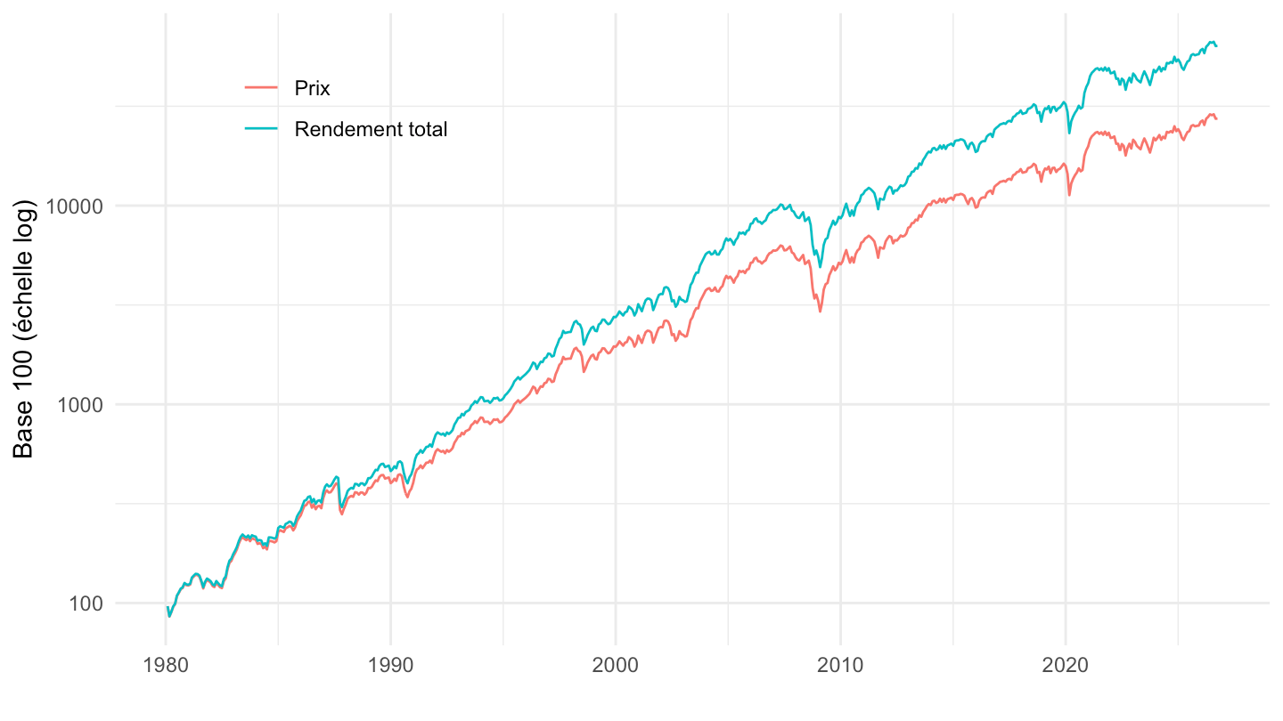
ew_l |> group_by(serie) |> summarise(Début = min(month), `Rendement annualisé (%)` = round(100 * (prod(1 + r)^(12 / n()) - 1), 2),
.groups = "drop") |> print_table_conditional()| serie | Début | Rendement annualisé (%) |
|---|---|---|
| Prix | 1980-02-01 | 12.76 |
| Rendement total | 1980-02-01 | 14.81 |
tibble(`Lignes` = nrow(adj), `Titres` = n_distinct(adj$ticker),
       `Adjusted <= 0` = sum(adj$Adjusted <= 0, na.rm = TRUE),
       `Titres concernés` = n_distinct(adj$ticker[adj$Adjusted <= 0 & !is.na(adj$Adjusted)]),
`Close <= 0` = sum(adj$Close <= 0, na.rm = TRUE)) |> print_table_conditional()| Lignes | Titres | Adjusted <= 0 | Titres concernés | Close <= 0 |
|---|---|---|---|---|
| 20034369 | 3073 | 3750 | 10 | 10 |
Les Adjusted <= 0 viennent d’un défaut de Yahoo (dividende exceptionnel supérieur au cours) : à écarter avant de calculer des rendements.