Code
WID_data_FR %>%
  group_by(variable, age, pop) %>%
  summarise(Nobs = n()) %>%
  arrange(-Nobs) %>%
print_table_conditional()Data
WID_data_FR %>%
group_by(variable, age, pop) %>%
summarise(Nobs = n()) %>%
arrange(-Nobs) %>%
print_table_conditional()WID_data_FR %>%
group_by(percentile) %>%
summarise(Nobs = n()) %>%
arrange(-Nobs) %>%
print_table_conditional()WID_metadata_FR %>%
mutate(type = substr(variable, 1, 1)) %>%
group_by(type, shorttype, longtype) %>%
summarise(Nobs = n()) %>%
arrange(-Nobs) %>%
print_table_conditional()| type | shorttype | longtype | Nobs |
|---|---|---|---|
| a | Average | Average income or wealth between two percentiles. When the associated percentile is of the form 'pX', intermediary average returns the average between percentile pX and the next consecutive percentile. When the associated percentile is of the form 'pXpY', the variable returns the average between percentiles pX and pY. | 678 |
| m | Total | Macroeconomic variable (i.e. corresponding to national economy rather than to a given group of individuals). The associated percentile is of the form 'pall'. | 327 |
| w | Wealth-income ratio | Ratio of net wealth (of a given sector) to net national income | 171 |
| n | Population | Number of units in a given group | 117 |
| e | Total emissions | Aggregrate emissions | 26 |
| k | Per-capita emissions | Per capita emissions | 26 |
| s | Share | Income or wealth shares. When the associated percentile is of the form 'pX', the raw data stores the share of total income or wealth detained by all the population between threshold pX and the top of the distribution. When the associated percentile is of the form 'pXpY', the raw data stores the share of the population between thresholds pX and pY. | 17 |
| t | Threshold | Percentile (i.e. threshold ) value at pX, whether the percentile is of the form 'pX' or of the form 'pXpY' | 17 |
| g | Gini coefficient | The Gini coefficient is a measure of statistical dispersion. A coefficient of zero expresses perfect equality between individuals. A coefficient of one expresses maximal inequality, where only one person owns all the income or wealth of the economy. | 15 |
| b | Beta coefficient | The beta coefficient corresponds to the inverted Pareto-Lorenz coefficient. It is equal to mean income over a certain income level divided by this level. A coefficient b=2=200% for an income level 100 000 EUR means that the average income above 100 000 EUR is 200 000 EUR, a coefficient of 3 or 300% at income level 1 000 000 EUR means that the average income level above 1 000 000 EUR in a given population is 3 000 000 EUR. | 14 |
| r | Top 10/Bottom 50 ratio | Ratio of Top 10% average income to Bottom 50% average income | 12 |
| x | Exchange rates | Exchange rate series | 6 |
| l | Average per capita group emissions | Average per capita group emissions for percentile pXpX+1 or PXpY | 4 |
| i | Indices | Indices | 3 |
| f | Female pop. | Female population size in a given group. | 1 |
| p | Proportion of women in group | Proportion of women in a given income or wealth group. The value of ppllin996i for the percentile group p90p100 corresponds to the proportion of women in the Top 10% earners in terms of pretax labor income | 1 |
WID_data_FR %>%
  left_join(age, by = "age") %>%
  group_by(age, shortage, longage) %>%
  summarise(Nobs = n()) %>%
  arrange(-Nobs) %>%
print_table_conditional()WID_data_FR %>%
left_join(pop, by = "pop") %>%
group_by(pop, shortpop, longpop) %>%
summarise(Nobs = n()) %>%
arrange(-Nobs) %>%
print_table_conditional()| pop | shortpop | longpop | Nobs |
|---|---|---|---|
| j | equal-split adults | The base unit is the individual (rather than the household) but resources are split equally within couples. | 544096 |
| i | individuals | The base unit is the individual (rather than the household). This is equivalent to assuming no sharing of resources within couples. | 223015 |
| t | tax unit | The base unit is the tax unit defined by national fiscal administrations to measure personal income taxes. | 187690 |
| m | male | The population looked at is comprised of male individuals only. | 80049 |
| f | female | The population looked at is comprised of female individuals only. | 78733 |
WID_data_FR %>%
  mutate(name = substr(variable, 2, 6)) %>%
  left_join(name, by = "name") %>%
  group_by(name, shortname, simpledes, technicaldes) %>%
  summarise(Nobs = n()) %>%
  arrange(-Nobs) %>%
  print_table_conditional()
country %>%
mutate(Flag = gsub(" ", "-", str_to_lower(gsub(" ", "-", Country))),
Flag = paste0('<img src="../../icon/flag/vsmall/', Flag, '.png" alt="Flag">')) %>%
select(Flag, everything()) %>%
{if (is_html_output()) datatable(., filter = 'top', rownames = F, escape = F) else .}WID_metadata_FR %>%
select(variable, shortname, shorttype, shortpop, shortage) %>%
print_table_conditionalWID_metadata_FR %>%
filter(grepl("Pre-tax", shortname)) %>%
select(variable, shortname, shorttype, shortpop, shortage) %>%
print_table_conditionalWID_metadata_FR %>%
filter(grepl("Post-tax", shortname)) %>%
select(variable, shortname, shorttype, shortpop, shortage) %>%
print_table_conditional| variable | shortname | shorttype | shortpop | shortage |
|---|---|---|---|---|
| acaincj992 | Post-tax disposable income | Average | equal-split adults | Adults |
| adiincj992 | Post-tax national income | Average | equal-split adults | Adults |
| bcaincj992 | Post-tax disposable income | Beta coefficient | equal-split adults | Adults |
| bdiincj992 | Post-tax national income | Beta coefficient | equal-split adults | Adults |
| gcaincj992 | Post-tax disposable income | Gini coefficient | equal-split adults | Adults |
| gdiincj992 | Post-tax national income | Gini coefficient | equal-split adults | Adults |
| rcaincj992 | Post-tax disposable income | Top 10/Bottom 50 ratio | equal-split adults | Adults |
| rdiincj992 | Post-tax national income | Top 10/Bottom 50 ratio | equal-split adults | Adults |
| scaincj992 | Post-tax disposable income | Share | equal-split adults | Adults |
| sdiincj992 | Post-tax national income | Share | equal-split adults | Adults |
| tcaincj992 | Post-tax disposable income | Threshold | equal-split adults | Adults |
| tdiincj992 | Post-tax national income | Threshold | equal-split adults | Adults |
WID_data_FR %>%
  filter(percentile == "p99.9p100") %>%
  group_by(variable, age, pop) %>%
  summarise(Nobs = n()) %>%
  arrange(-Nobs) %>%
print_table_conditionalload_data("wid/name_fr.RData")
WID_data_FR %>%
bind_rows(WID_data_GB) %>%
mutate(name = substr(variable, 2, 6),
type = substr(variable, 1, 1)) %>%
filter(name %in% c("ptinc", "diinc"),
type == "s",
pop == "j",
percentile %in% c("p90p100")) %>%
year_to_date2() %>%
filter(date >= as.Date("1914-01-01")) %>%
left_join(country, by = "country") %>%
left_join(name, by = "name") %>%
rename(Location = Country) %>%
left_join(colors, by = c("Location" = "country")) %>%
ggplot + geom_line(aes(x = date, y = value, color = color, linetype = shortname)) +
scale_color_identity() + ylab("Part du revenu national du 10% les + riches (%)") +
xlab("") + theme_minimal() + add_4flags +
scale_y_continuous(breaks = 0.01*seq(0, 100, 2),
labels = scales::percent_format(accuracy = 1)) +
scale_x_date(breaks = seq(1800, 2025, 10) %>% paste0("-01-01") %>% as.Date,
labels = date_format("%Y")) +
theme(legend.position = c(0.6, 0.9),
legend.title = element_blank())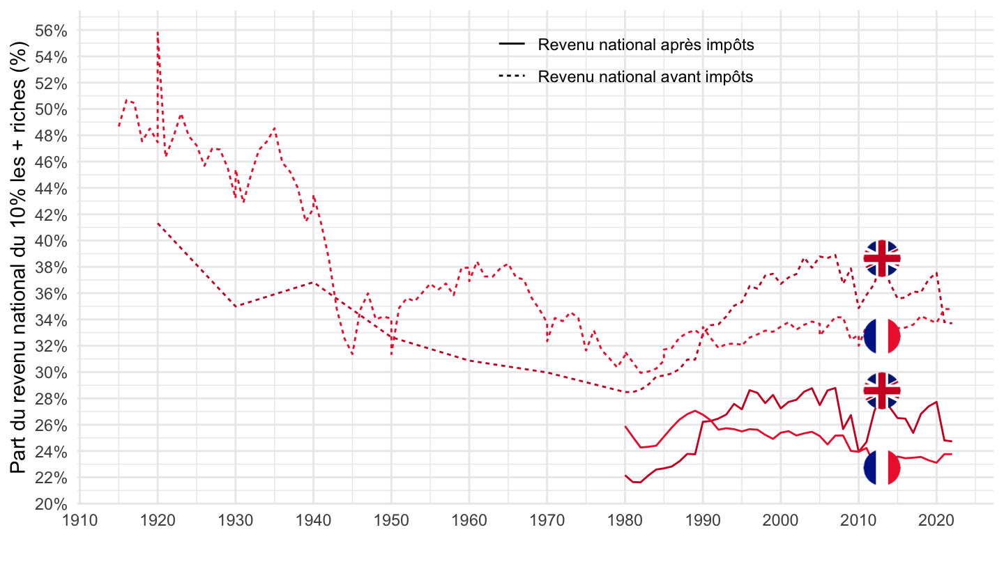
WID_data_DE %>%
  bind_rows(WID_data_FR) %>%
  bind_rows(WID_data_GB) %>%
  mutate(name = substr(variable, 2, 6),
         type = substr(variable, 1, 1)) %>%
  filter(name %in% c("ptinc", "diinc"),
         type == "s",
         pop == "j",
         percentile %in% c("p99p100"),
         country %in% c("FR", "GB")) %>%
  year_to_date2() %>%
  filter(date >= as.Date("1914-01-01")) %>%
  left_join(country, by = "country") %>%
  left_join(name, by = "name") %>%
  rename(Location = Country) %>%
  left_join(colors, by = c("Location" = "country")) %>%

  ggplot + geom_line(aes(x = date, y = value, color = color, linetype = shortname)) +
  scale_color_identity() + ylab("Part du revenu national du 1% les + riches (%)") +
  xlab("") + theme_minimal() + add_4flags +
  scale_y_continuous(breaks = 0.01*seq(0, 100, 2),
                     labels = scales::percent_format(accuracy = 1)) +
  scale_x_date(breaks = seq(1800, 2025, 10) %>% paste0("-01-01") %>% as.Date,
               labels = date_format("%Y")) +
  theme(legend.position = c(0.6, 0.9),
        legend.title = element_blank())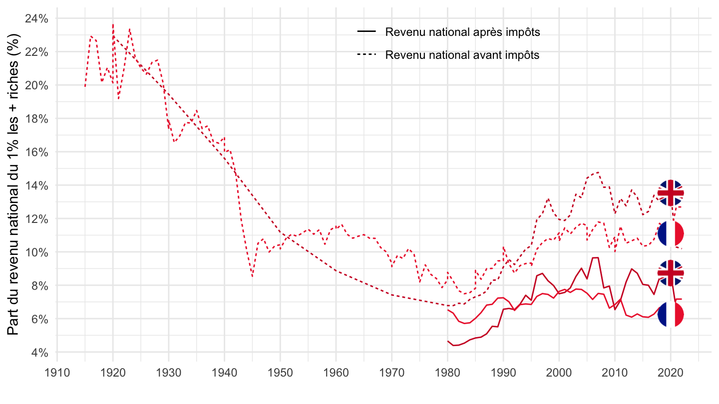
WID_data_DE %>%
  bind_rows(WID_data_FR) %>%
  bind_rows(WID_data_GB) %>%
  mutate(name = substr(variable, 2, 6),
         type = substr(variable, 1, 1)) %>%
  filter(name %in% c("ptinc", "diinc"),
         type == "s",
         pop == "j",
         percentile %in% c("p99.9p100"),
         country %in% c("FR", "GB")) %>%
  year_to_date2() %>%
  filter(date >= as.Date("1914-01-01")) %>%
  left_join(country, by = "country") %>%
  left_join(name, by = "name") %>%
  rename(Location = Country) %>%
  left_join(colors, by = c("Location" = "country")) %>%

  ggplot + geom_line(aes(x = date, y = value, color = color, linetype = shortname)) +
  scale_color_identity() + ylab("Part du revenu national du 0.1% les + riches (%)") +
  xlab("") + theme_minimal() + add_4flags +
  scale_y_continuous(breaks = 0.01*seq(0, 100, 2),
                     labels = scales::percent_format(accuracy = 1)) +
  scale_x_date(breaks = seq(1800, 2025, 10) %>% paste0("-01-01") %>% as.Date,
               labels = date_format("%Y")) +
  theme(legend.position = c(0.6, 0.9),
        legend.title = element_blank())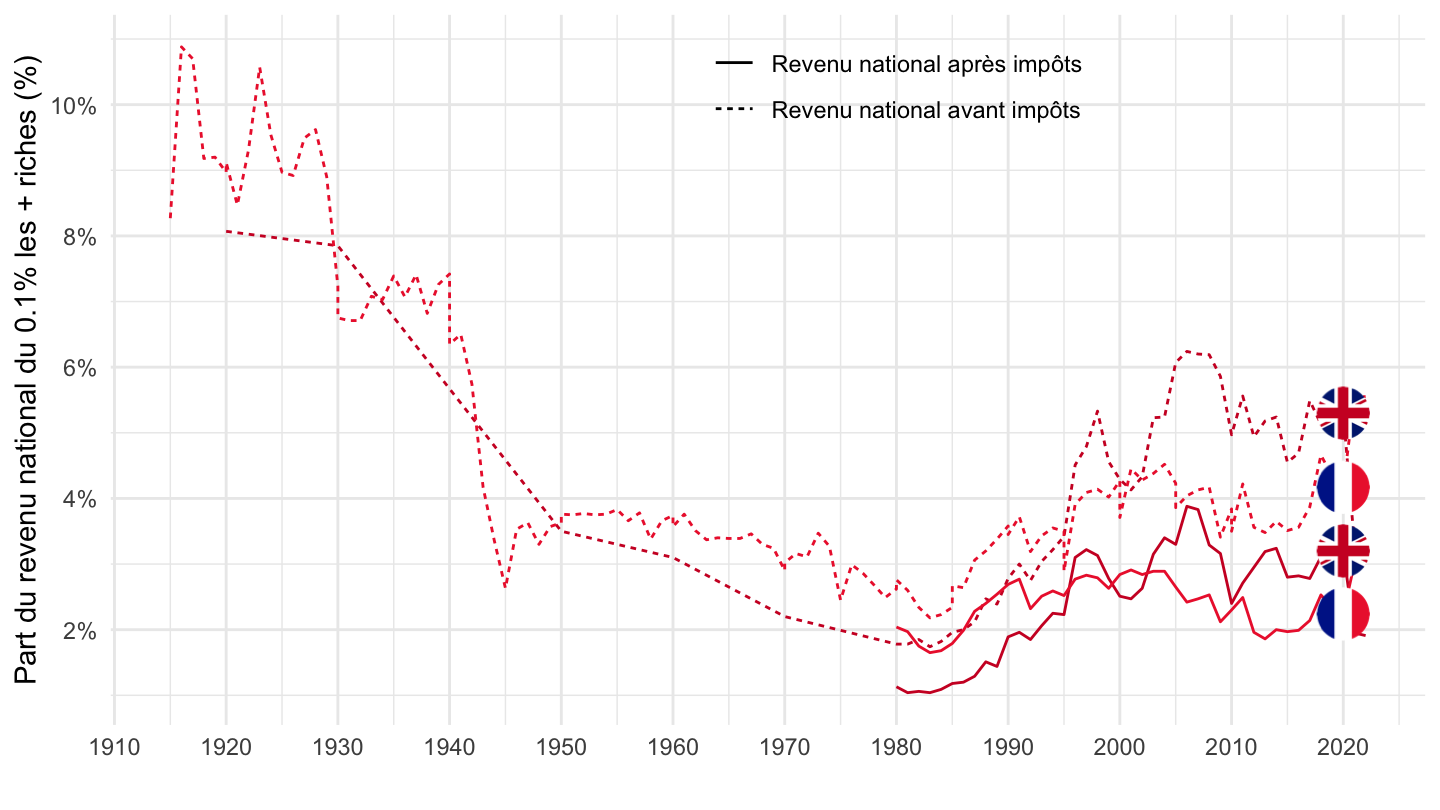
WID_data_DE %>%
  bind_rows(WID_data_FR) %>%
  bind_rows(WID_data_GB) %>%
  mutate(name = substr(variable, 2, 6),
         type = substr(variable, 1, 1)) %>%
  filter(name %in% c("ptinc", "diinc"),
         type == "s",
         pop == "j",
         percentile %in% c("p99.99p100"),
         country %in% c("FR", "GB")) %>%
  year_to_date2() %>%
  filter(date >= as.Date("1914-01-01")) %>%
  left_join(country, by = "country") %>%
  left_join(name, by = "name") %>%
  rename(Location = Country) %>%
  left_join(colors, by = c("Location" = "country")) %>%

  ggplot + geom_line(aes(x = date, y = value, color = color, linetype = shortname)) +
  scale_color_identity() + ylab("Part du revenu national du 0.01% les + riches (%)") +
  xlab("") + theme_minimal() + add_4flags +
  scale_y_continuous(breaks = 0.01*seq(0, 100, 1),
                     labels = scales::percent_format(accuracy = 1)) +
  scale_x_date(breaks = seq(1800, 2025, 10) %>% paste0("-01-01") %>% as.Date,
               labels = date_format("%Y")) +
  theme(legend.position = c(0.6, 0.9),
        legend.title = element_blank())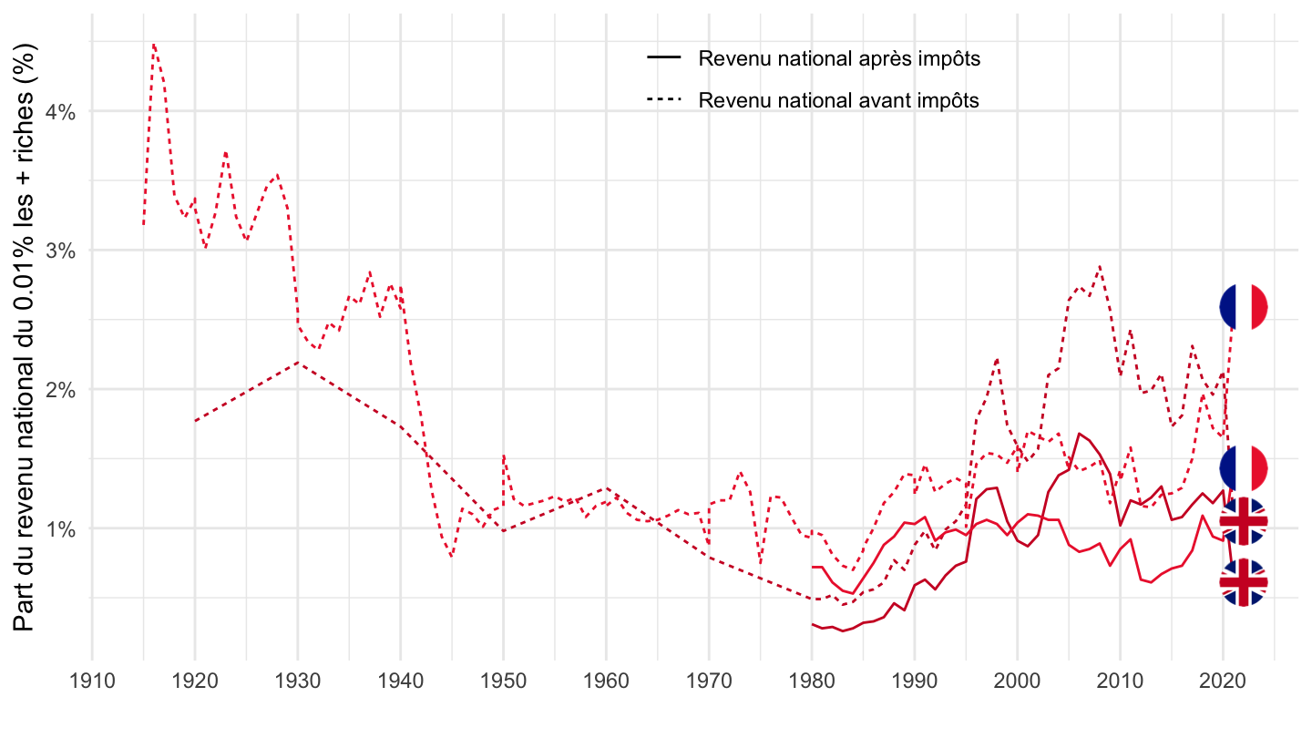
WID_data_DE %>%
  bind_rows(WID_data_FR) %>%
  bind_rows(WID_data_GB) %>%
  mutate(name = substr(variable, 2, 6),
         type = substr(variable, 1, 1)) %>%
  filter(name %in% c("ptinc", "diinc"),
         type == "s",
         pop == "j",
         percentile %in% c("p99.99p100"),
         country %in% c("FR", "GB")) %>%
  year_to_date2() %>%
  filter(date >= as.Date("1980-01-01")) %>%
  left_join(country, by = "country") %>%
  left_join(name, by = "name") %>%
  rename(Location = Country) %>%
  left_join(colors, by = c("Location" = "country")) %>%

  ggplot + geom_line(aes(x = date, y = value, color = color, linetype = shortname)) +
  scale_color_identity() + ylab("Part du revenu national du 0.01% les + riches (%)") +
  xlab("") + theme_minimal() + add_4flags +
  scale_y_continuous(breaks = 0.01*seq(0, 100, .2),
                     labels = scales::percent_format(accuracy = .1)) +
  scale_x_date(breaks = seq(1800, 2025, 5) %>% paste0("-01-01") %>% as.Date,
               labels = date_format("%Y")) +
  theme(legend.position = c(0.2, 0.9),
        legend.title = element_blank())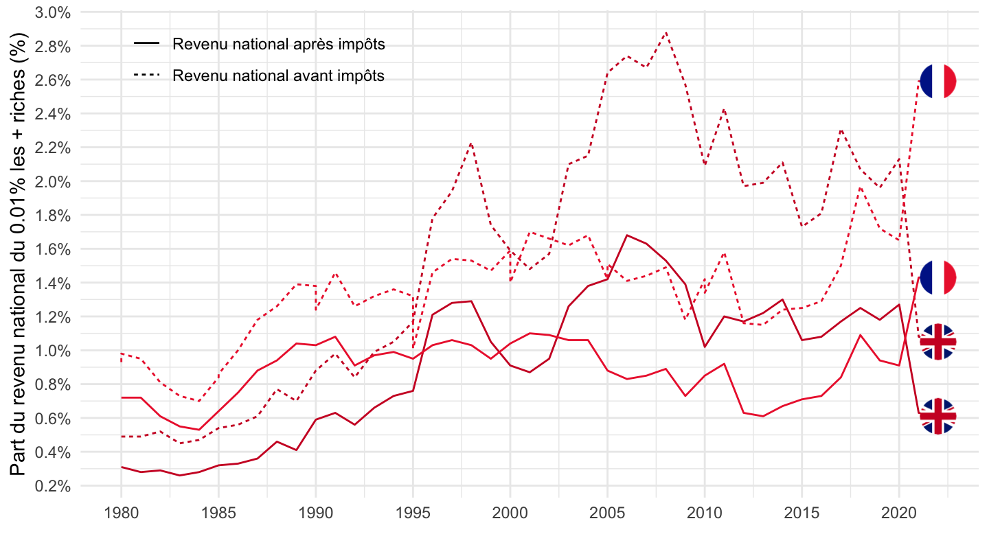
WID_data_DE %>%
  bind_rows(WID_data_FR) %>%
  bind_rows(WID_data_GB) %>%
  mutate(name = substr(variable, 2, 6),
         type = substr(variable, 1, 1)) %>%
  filter(name %in% c("ptinc", "diinc"),
         type == "s",
         pop == "j",
         percentile %in% c("p99.999p100"),
         country %in% c("FR", "GB")) %>%
  year_to_date2() %>%
  filter(date >= as.Date("1914-01-01")) %>%
  left_join(country, by = "country") %>%
  left_join(name, by = "name") %>%
  rename(Location = Country) %>%
  left_join(colors, by = c("Location" = "country")) %>%

  ggplot + geom_line(aes(x = date, y = value, color = color, linetype = shortname)) +
  scale_color_identity() + ylab("Part du revenu national du 0.001% les + riches (%)") +
  xlab("") + theme_minimal() + add_4flags +
  scale_y_continuous(breaks = 0.01*seq(0, 100, 1),
                     labels = scales::percent_format(accuracy = 1)) +
  scale_x_date(breaks = seq(1800, 2025, 10) %>% paste0("-01-01") %>% as.Date,
               labels = date_format("%Y")) +
  theme(legend.position = c(0.6, 0.9),
        legend.title = element_blank())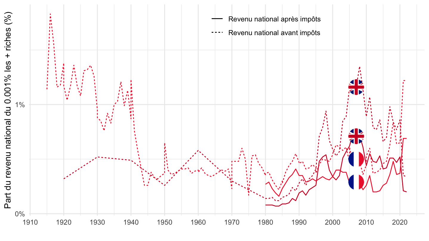
WID_data_QY %>%
  bind_rows(WID_data_US) %>%
  mutate(name = substr(variable, 2, 6),
         type = substr(variable, 1, 1)) %>%
  filter(name %in% c("ptinc", "diinc"),
         type == "s",
         pop == "j",
         percentile %in% c("p90p100")) %>%
  year_to_date2() %>%
  filter(date >= as.Date("1914-01-01")) %>%
  left_join(country, by = "country") %>%
  left_join(name, by = "name") %>%
  rename(Location = Country) %>%
  left_join(colors, by = c("Location" = "country")) %>%
  mutate(color = ifelse(Location == "United States", color2, color)) %>%
  ggplot + geom_line(aes(x = date, y = value, color = color, linetype = shortname)) +
  scale_color_identity() + ylab("Part du revenu national du 10% les + riches (%)") +
  xlab("") + theme_minimal() + add_4flags +
  scale_y_continuous(breaks = 0.01*seq(0, 100, 2),
                     labels = scales::percent_format(accuracy = 1)) +
  scale_x_date(breaks = seq(1800, 2025, 10) %>% paste0("-01-01") %>% as.Date,
               labels = date_format("%Y")) +
  theme(legend.position = c(0.6, 0.9),
        legend.title = element_blank())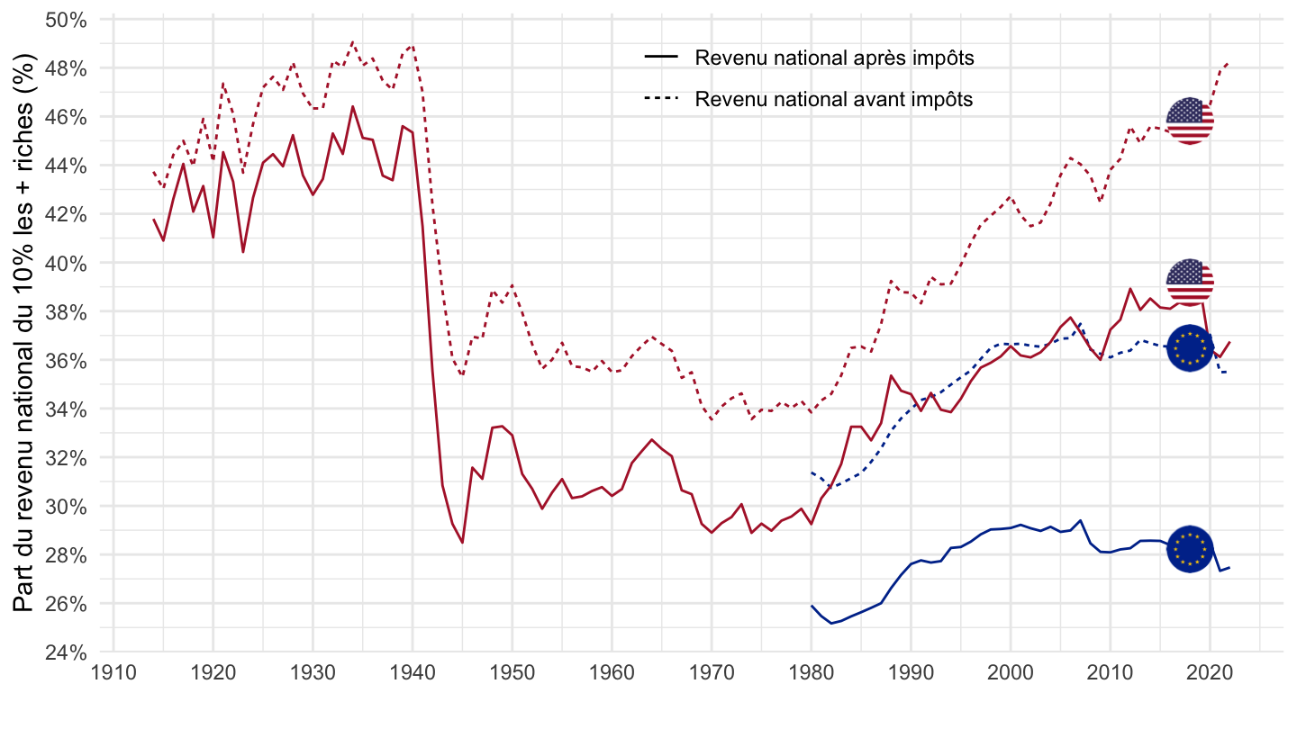
WID_data_QY %>%
  bind_rows(WID_data_US) %>%
  mutate(name = substr(variable, 2, 6),
         type = substr(variable, 1, 1)) %>%
  filter(name %in% c("ptinc", "diinc"),
         type == "s",
         pop == "j",
         percentile %in% c("p90p100")) %>%
  year_to_date2() %>%
  filter(date >= as.Date("1980-01-01")) %>%
  left_join(country, by = "country") %>%
  left_join(name, by = "name") %>%
  rename(Location = Country) %>%
  left_join(colors, by = c("Location" = "country")) %>%
  mutate(color = ifelse(Location == "United States", color2, color)) %>%
  ggplot + geom_line(aes(x = date, y = value, color = color, linetype = shortname)) +
  scale_color_identity() + ylab("Part du revenu national du 10% les + riches (%)") +
  xlab("") + theme_minimal() + add_4flags +
  scale_y_continuous(breaks = 0.01*seq(0, 100, 2),
                     labels = scales::percent_format(accuracy = 1)) +
  scale_x_date(breaks = c(seq(1979, 2100, 5), seq(1977, 2100, 5)) %>% paste0("-01-01") %>% as.Date,
               labels = date_format("%Y")) +
  theme(legend.position = c(0.6, 0.9),
        legend.title = element_blank())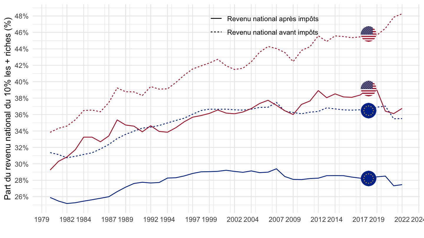
WID_data_QY %>%
  bind_rows(WID_data_US) %>%
  mutate(name = substr(variable, 2, 6),
         type = substr(variable, 1, 1)) %>%
  filter(name %in% c("ptinc", "diinc"),
         type == "s",
         pop == "j",
         percentile %in% c("p90p100")) %>%
  year_to_date2() %>%
  filter(date >= as.Date("1999-01-01")) %>%
  left_join(country, by = "country") %>%
  left_join(name, by = "name") %>%
  rename(Location = Country) %>%
  left_join(colors, by = c("Location" = "country")) %>%
  mutate(color = ifelse(Location == "United States", color2, color)) %>%
  ggplot + geom_line(aes(x = date, y = value, color = color, linetype = shortname)) +
  scale_color_identity() + ylab("Part du revenu national du 10% les + riches (%)") +
  xlab("") + theme_minimal() + add_4flags +
  scale_y_continuous(breaks = 0.01*seq(0, 100, 2),
                     labels = scales::percent_format(accuracy = 1)) +
  scale_x_date(breaks = c(seq(1999, 2100, 5), seq(1997, 2100, 5)) %>% paste0("-01-01") %>% as.Date,
               labels = date_format("%Y")) +
  theme(legend.position = c(0.2, 0.9),
        legend.title = element_blank())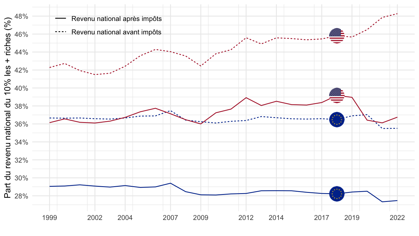
WID_data_QY %>%
  bind_rows(WID_data_US) %>%
  mutate(name = substr(variable, 2, 6),
         type = substr(variable, 1, 1)) %>%
  filter(name %in% c("ptinc", "diinc"),
         type == "s",
         pop == "j",
         percentile %in% c("p99p100")) %>%
  year_to_date2() %>%
  filter(date >= as.Date("1914-01-01")) %>%
  left_join(country, by = "country") %>%
  left_join(name, by = "name") %>%
  rename(Location = Country) %>%
  left_join(colors, by = c("Location" = "country")) %>%

  ggplot + geom_line(aes(x = date, y = value, color = color, linetype = shortname)) +
  scale_color_identity() + ylab("Part du revenu national du 1% les + riches (%)") +
  xlab("") + theme_minimal() + add_4flags +
  scale_y_continuous(breaks = 0.01*seq(0, 100, 2),
                     labels = scales::percent_format(accuracy = 1)) +
  scale_x_date(breaks = seq(1800, 2025, 10) %>% paste0("-01-01") %>% as.Date,
               labels = date_format("%Y")) +
  theme(legend.position = c(0.6, 0.9),
        legend.title = element_blank())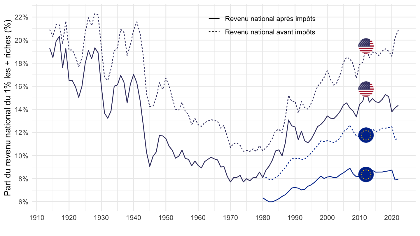
WID_data_QY %>%
  bind_rows(WID_data_US) %>%
  mutate(name = substr(variable, 2, 6),
         type = substr(variable, 1, 1)) %>%
  filter(name %in% c("ptinc", "diinc"),
         type == "s",
         pop == "j",
         percentile %in% c("p99.9p100")) %>%
  year_to_date2() %>%
  filter(date >= as.Date("1914-01-01")) %>%
  left_join(country, by = "country") %>%
  left_join(name, by = "name") %>%
  rename(Location = Country) %>%
  left_join(colors, by = c("Location" = "country")) %>%

  ggplot + geom_line(aes(x = date, y = value, color = color, linetype = shortname)) +
  scale_color_identity() + ylab("Part du revenu national du 0.1% les + riches (%)") +
  xlab("") + theme_minimal() + add_4flags +
  scale_y_continuous(breaks = 0.01*seq(0, 100, 1),
                     labels = scales::percent_format(accuracy = 1)) +
  scale_x_date(breaks = seq(1800, 2025, 10) %>% paste0("-01-01") %>% as.Date,
               labels = date_format("%Y")) +
  theme(legend.position = c(0.6, 0.9),
        legend.title = element_blank())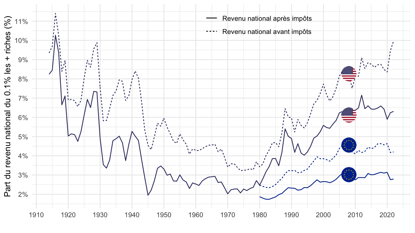
WID_data_QY %>%
  bind_rows(WID_data_US) %>%
  mutate(name = substr(variable, 2, 6),
         type = substr(variable, 1, 1)) %>%
  filter(name %in% c("ptinc", "diinc"),
         type == "s",
         pop == "j",
         percentile %in% c("p99.99p100")) %>%
  year_to_date2() %>%
  filter(date >= as.Date("1914-01-01")) %>%
  left_join(country, by = "country") %>%
  left_join(name, by = "name") %>%
  rename(Location = Country) %>%
  left_join(colors, by = c("Location" = "country")) %>%

  ggplot + geom_line(aes(x = date, y = value, color = color, linetype = shortname)) +
  scale_color_identity() + ylab("Part du revenu national du 0.01% les + riches (%)") +
  xlab("") + theme_minimal() + add_4flags +
  scale_y_continuous(breaks = 0.01*seq(0, 100, 1),
                     labels = scales::percent_format(accuracy = 1)) +
  scale_x_date(breaks = seq(1800, 2025, 10) %>% paste0("-01-01") %>% as.Date,
               labels = date_format("%Y")) +
  theme(legend.position = c(0.6, 0.9),
        legend.title = element_blank())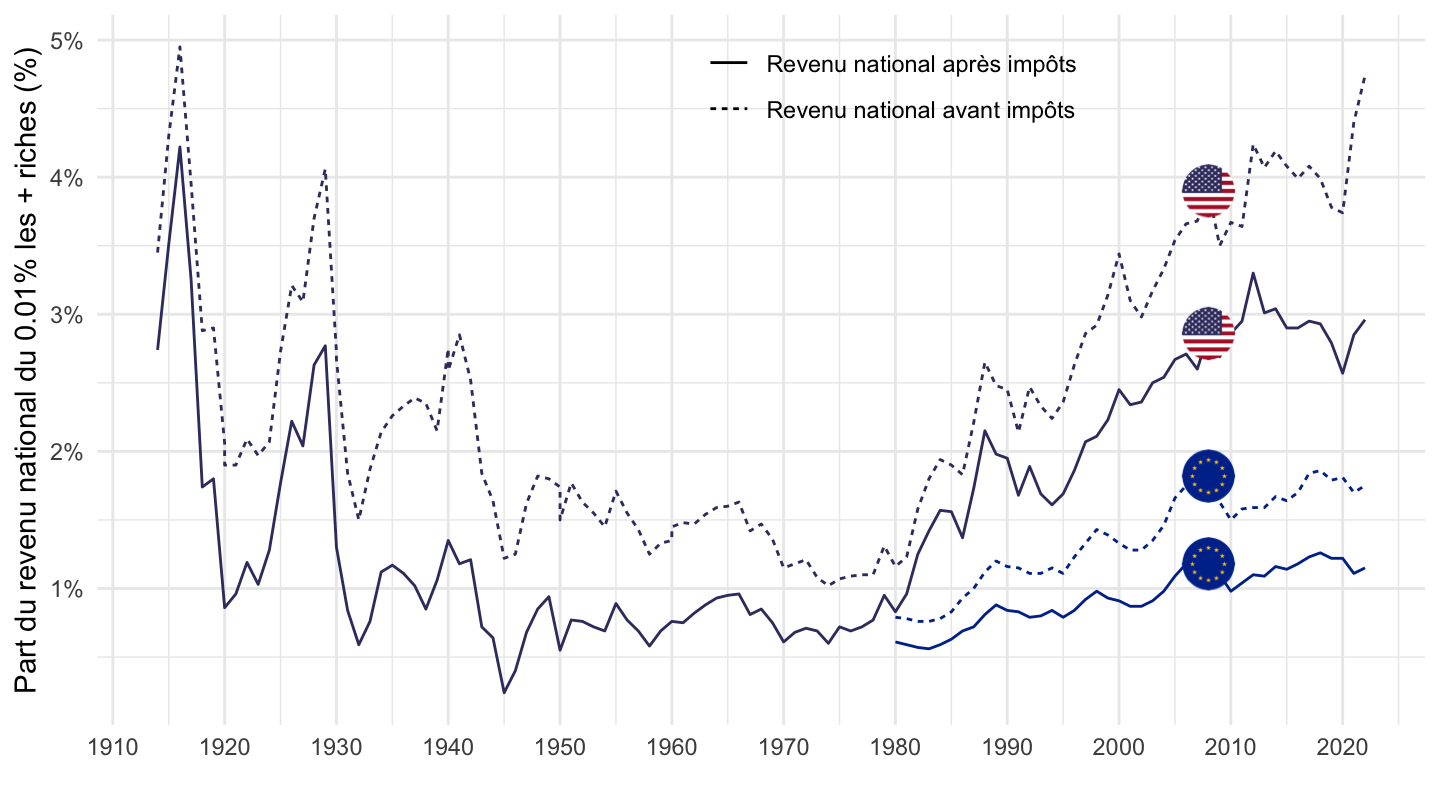
WID_data_QY %>%
  bind_rows(WID_data_US) %>%
  mutate(name = substr(variable, 2, 6),
         type = substr(variable, 1, 1)) %>%
  filter(name %in% c("ptinc", "diinc"),
         type == "s",
         pop == "j",
         percentile %in% c("p99.999p100")) %>%
  year_to_date2() %>%
  filter(date >= as.Date("1914-01-01")) %>%
  left_join(country, by = "country") %>%
  left_join(name, by = "name") %>%
  rename(Location = Country) %>%
  left_join(colors, by = c("Location" = "country")) %>%

  ggplot + geom_line(aes(x = date, y = value, color = color, linetype = shortname)) +
  scale_color_identity() + ylab("Part du revenu national du 0.001% les + riches (%)") +
  xlab("") + theme_minimal() + add_4flags +
  scale_y_continuous(breaks = 0.01*seq(0, 100, 1),
                     labels = scales::percent_format(accuracy = 1)) +
  scale_x_date(breaks = seq(1800, 2025, 10) %>% paste0("-01-01") %>% as.Date,
               labels = date_format("%Y")) +
  theme(legend.position = c(0.6, 0.9),
        legend.title = element_blank())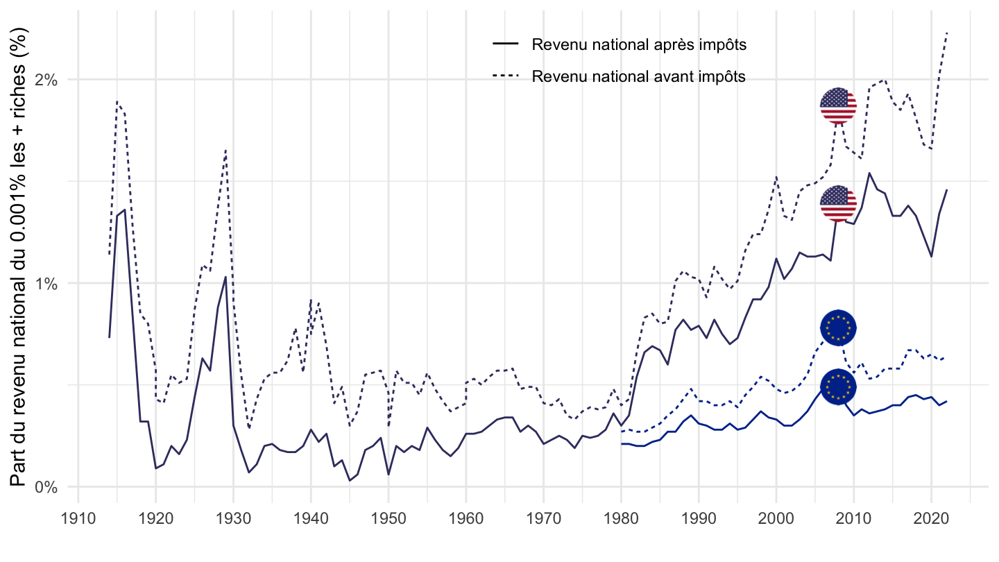
WID_data_DE %>%
  bind_rows(WID_data_FR) %>%
  bind_rows(WID_data_US) %>%
  mutate(name = substr(variable, 2, 6),
         type = substr(variable, 1, 1)) %>%
  filter(name %in% c("ptinc", "diinc"),
         type == "s",
         pop == "j",
         percentile %in% c("p90p100"),
         country %in% c("FR", "US")) %>%
  year_to_date2() %>%
  filter(date >= as.Date("1914-01-01")) %>%
  left_join(country, by = "country") %>%
  left_join(name, by = "name") %>%
  rename(Location = Country) %>%
  left_join(colors, by = c("Location" = "country")) %>%
  ggplot + geom_line(aes(x = date, y = value, color = color, linetype = shortname)) +
  scale_color_identity() + ylab("Part du revenu national du 10% les + riches (%)") +
  xlab("") + theme_minimal() + add_4flags +
  scale_y_continuous(breaks = 0.01*seq(0, 100, 2),
                     labels = scales::percent_format(accuracy = 1)) +
  scale_x_date(breaks = seq(1800, 2025, 10) %>% paste0("-01-01") %>% as.Date,
               labels = date_format("%Y")) +
  theme(legend.position = c(0.6, 0.9),
        legend.title = element_blank())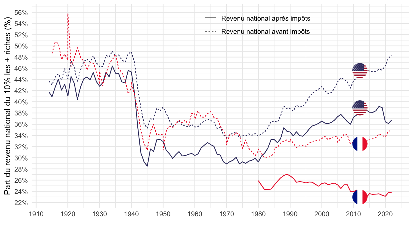
WID_data_DE %>%
  bind_rows(WID_data_FR) %>%
  bind_rows(WID_data_US) %>%
  mutate(name = substr(variable, 2, 6),
         type = substr(variable, 1, 1)) %>%
  filter(name %in% c("ptinc", "diinc"),
         type == "s",
         pop == "j",
         percentile %in% c("p99p100"),
         country %in% c("FR", "US")) %>%
  year_to_date2() %>%
  filter(date >= as.Date("1914-01-01")) %>%
  left_join(country, by = "country") %>%
  left_join(name, by = "name") %>%
  rename(Location = Country) %>%
  left_join(colors, by = c("Location" = "country")) %>%
  ggplot + geom_line(aes(x = date, y = value, color = color, linetype = shortname)) +
  scale_color_identity() + ylab("Part du revenu national du 1% les + riches (%)") +
  xlab("") + theme_minimal() + add_4flags +
  scale_y_continuous(breaks = 0.01*seq(0, 100, 2),
                     labels = scales::percent_format(accuracy = 1)) +
  scale_x_date(breaks = seq(1800, 2025, 10) %>% paste0("-01-01") %>% as.Date,
               labels = date_format("%Y")) +
  theme(legend.position = c(0.6, 0.9),
        legend.title = element_blank())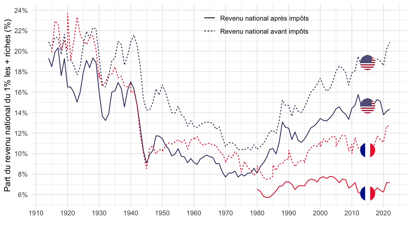
WID_data_DE %>%
  bind_rows(WID_data_FR) %>%
  bind_rows(WID_data_US) %>%
  mutate(name = substr(variable, 2, 6),
         type = substr(variable, 1, 1)) %>%
  filter(name %in% c("ptinc", "diinc"),
         type == "s",
         pop == "j",
         percentile %in% c("p99p100"),
         country %in% c("FR", "US")) %>%
  year_to_date2() %>%
  filter(date >= as.Date("1999-01-01")) %>%
  left_join(country, by = "country") %>%
  left_join(name, by = "name") %>%
  rename(Location = Country) %>%
  left_join(colors, by = c("Location" = "country")) %>%
  ggplot + geom_line(aes(x = date, y = value, color = color, linetype = shortname)) +
  scale_color_identity() + ylab("Part du revenu national du 1% les + riches (%)") +
  xlab("") + theme_minimal() + add_4flags +
  scale_y_continuous(breaks = 0.01*seq(0, 100, 2),
                     labels = scales::percent_format(accuracy = 1)) +
  scale_x_date(breaks = seq(1999, 2025, 5) %>% paste0("-01-01") %>% as.Date,
               labels = date_format("%Y")) +
  theme(legend.position = c(0.6, 0.9),
        legend.title = element_blank())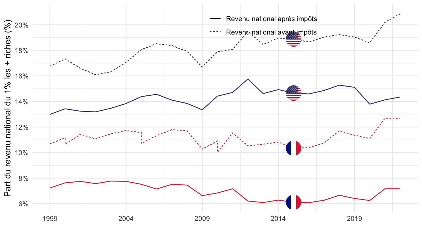
load_data("wid/name_fr.RData")
WID_data_DE %>%
  bind_rows(WID_data_FR) %>%
  bind_rows(WID_data_US) %>%
  mutate(name = substr(variable, 2, 6),
         type = substr(variable, 1, 1)) %>%
  filter(name %in% c("ptinc", "diinc"),
         type == "s",
         pop == "j",
         percentile %in% c("p99.9p100"),
         country %in% c("FR", "US")) %>%
  year_to_date2() %>%
  filter(date >= as.Date("1914-01-01")) %>%
  left_join(country, by = "country") %>%
  left_join(name, by = "name") %>%
  rename(Location = Country) %>%
  left_join(colors, by = c("Location" = "country")) %>%
  ggplot + geom_line(aes(x = date, y = value, color = color, linetype = shortname)) +
  scale_color_identity() + ylab("Part du revenu national du 0.1% les + riches (%)") +
  xlab("") + theme_minimal() + add_4flags +
  scale_y_continuous(breaks = 0.01*seq(0, 100, 1),
                     labels = scales::percent_format(accuracy = 1)) +
  scale_x_date(breaks = seq(1800, 2025, 10) %>% paste0("-01-01") %>% as.Date,
               labels = date_format("%Y")) +
  theme(legend.position = c(0.6, 0.9),
        legend.title = element_blank())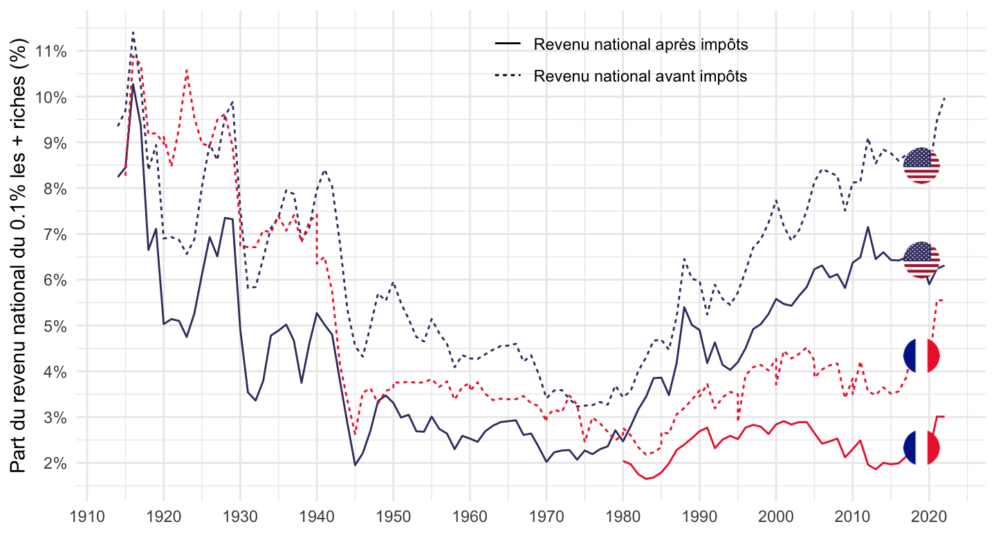
WID_data_DE %>%
  bind_rows(WID_data_FR) %>%
  bind_rows(WID_data_US) %>%
  mutate(name = substr(variable, 2, 6),
         type = substr(variable, 1, 1)) %>%
  filter(name %in% c("ptinc", "diinc"),
         type == "s",
         pop == "j",
         percentile %in% c("p99.99p100"),
         country %in% c("FR", "US")) %>%
  year_to_date2() %>%
  filter(date >= as.Date("1914-01-01")) %>%
  left_join(country, by = "country") %>%
  left_join(name, by = "name") %>%
  rename(Location = Country) %>%
  left_join(colors, by = c("Location" = "country")) %>%
  ggplot + geom_line(aes(x = date, y = value, color = color, linetype = shortname)) +
  scale_color_identity() + ylab("Part du revenu national du 0.01% les + riches (%)") +
  xlab("") + theme_minimal() + add_4flags +
  scale_y_continuous(breaks = 0.01*seq(0, 100, 1),
                     labels = scales::percent_format(accuracy = 1)) +
  scale_x_date(breaks = seq(1800, 2025, 10) %>% paste0("-01-01") %>% as.Date,
               labels = date_format("%Y")) +
  theme(legend.position = c(0.6, 0.9),
        legend.title = element_blank())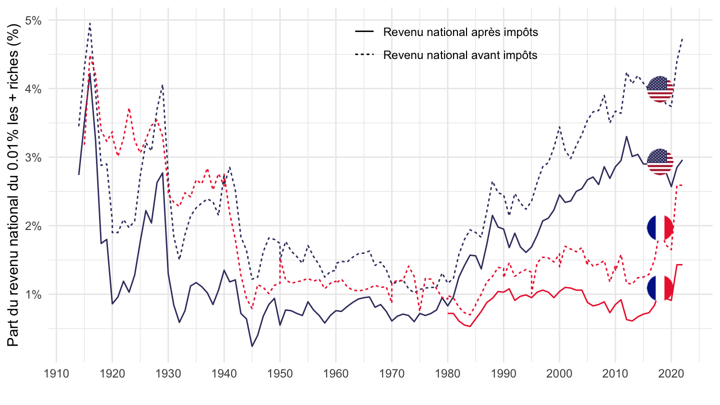
WID_data_DE %>%
  bind_rows(WID_data_FR) %>%
  bind_rows(WID_data_US) %>%
  mutate(name = substr(variable, 2, 6),
         type = substr(variable, 1, 1)) %>%
  filter(name %in% c("ptinc", "diinc"),
         type == "s",
         pop == "j",
         percentile %in% c("p99.999p100"),
         country %in% c("FR", "US")) %>%
  year_to_date2() %>%
  filter(date >= as.Date("1914-01-01")) %>%
  left_join(country, by = "country") %>%
  left_join(name, by = "name") %>%
  rename(Location = Country) %>%
  left_join(colors, by = c("Location" = "country")) %>%
  ggplot + geom_line(aes(x = date, y = value, color = color, linetype = shortname)) +
  scale_color_identity() + ylab("Part du revenu national du 0.001% les + riches (%)") +
  xlab("") + theme_minimal() + add_4flags +
  scale_y_continuous(breaks = 0.01*seq(0, 100, .2),
                     labels = scales::percent_format(accuracy = .1)) +
  scale_x_date(breaks = seq(1800, 2025, 10) %>% paste0("-01-01") %>% as.Date,
               labels = date_format("%Y")) +
  theme(legend.position = c(0.6, 0.9),
        legend.title = element_blank())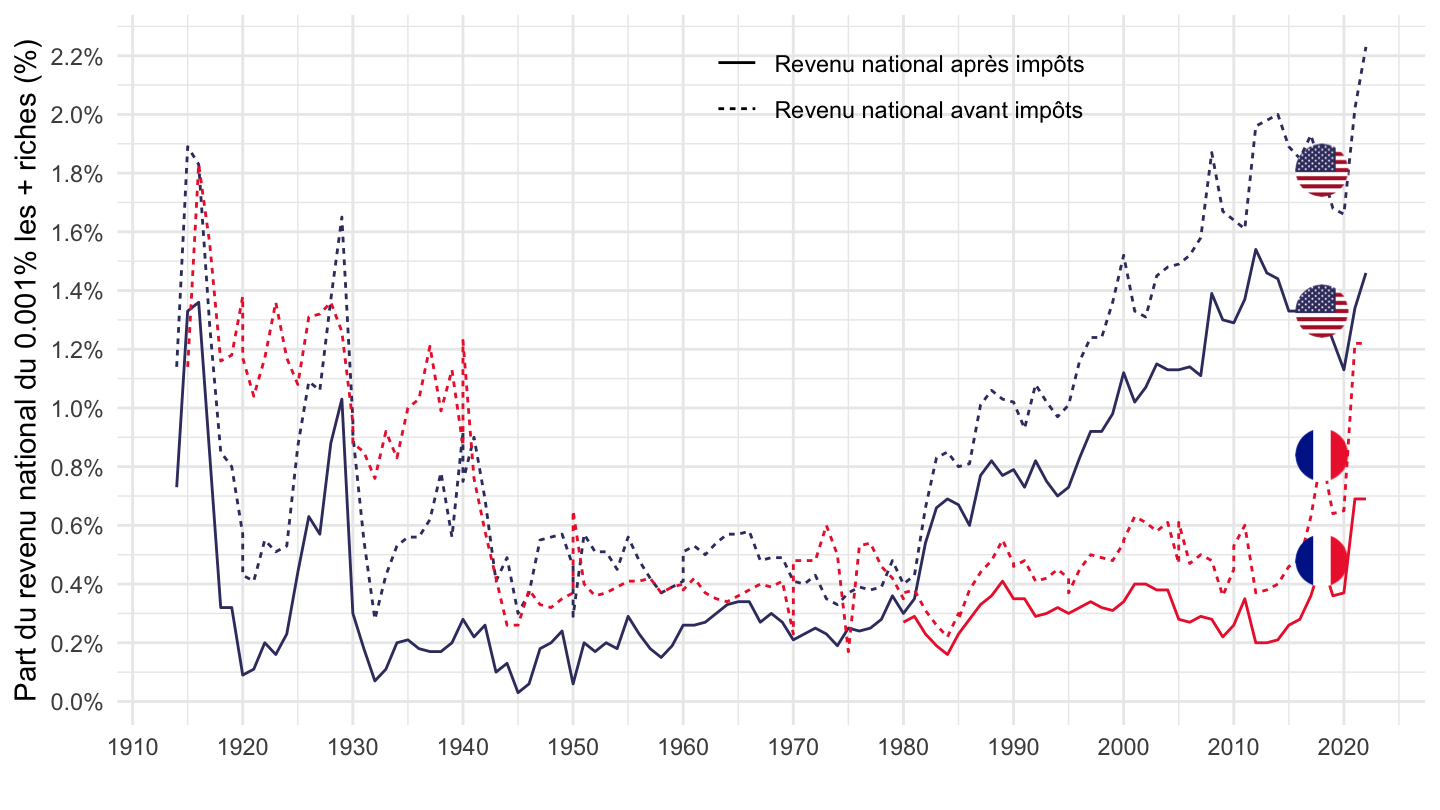
WID_data_DE %>%
  bind_rows(WID_data_FR) %>%
  bind_rows(WID_data_US) %>%
  mutate(name = substr(variable, 2, 6),
         type = substr(variable, 1, 1)) %>%
  filter(name %in% c("ptinc", "diinc"),
         type == "s",
         pop == "j",
         percentile %in% c("p99p100", "p90p100"),
         country %in% c("FR", "US")) %>%
  year_to_date2() %>%
  filter(date >= as.Date("1914-01-01")) %>%
  left_join(country, by = "country") %>%
  left_join(name, by = "name") %>%
  rename(Location = Country) %>%
  left_join(colors, by = c("Location" = "country")) %>%
  ggplot + geom_line(aes(x = date, y = value, color = color, linetype = shortname, linetype2 = percentile)) +
  scale_color_identity() + ylab("Part du revenu national (%)") + xlab("") + theme_minimal() +
  add_8flags +
  scale_y_continuous(breaks = 0.01*seq(0, 100, 5),
                     labels = scales::percent_format(accuracy = 1)) +
  scale_x_date(breaks = seq(1800, 2025, 10) %>% paste0("-01-01") %>% as.Date,
               labels = date_format("%Y")) +
  theme(legend.position = c(0.6, 0.9),
        legend.title = element_blank()) +
 annotate(geom="text", x = as.Date("1925-01-01"), y = 0.08, label = "par les 1% les + riches", size=3, fontface="bold") +
 annotate(geom="text", x = as.Date("1925-01-01"), y = 0.10, label = "Part du revenu détenue", size=3, fontface="bold") +
 annotate(geom="text", x = as.Date("1926-01-01"), y = 0.34, label = "par les 10% les + riches", size=3, fontface="bold") +
 annotate(geom="text", x = as.Date("1926-01-01"), y = 0.36, label = "Part du revenu détenue", size=3, fontface="bold")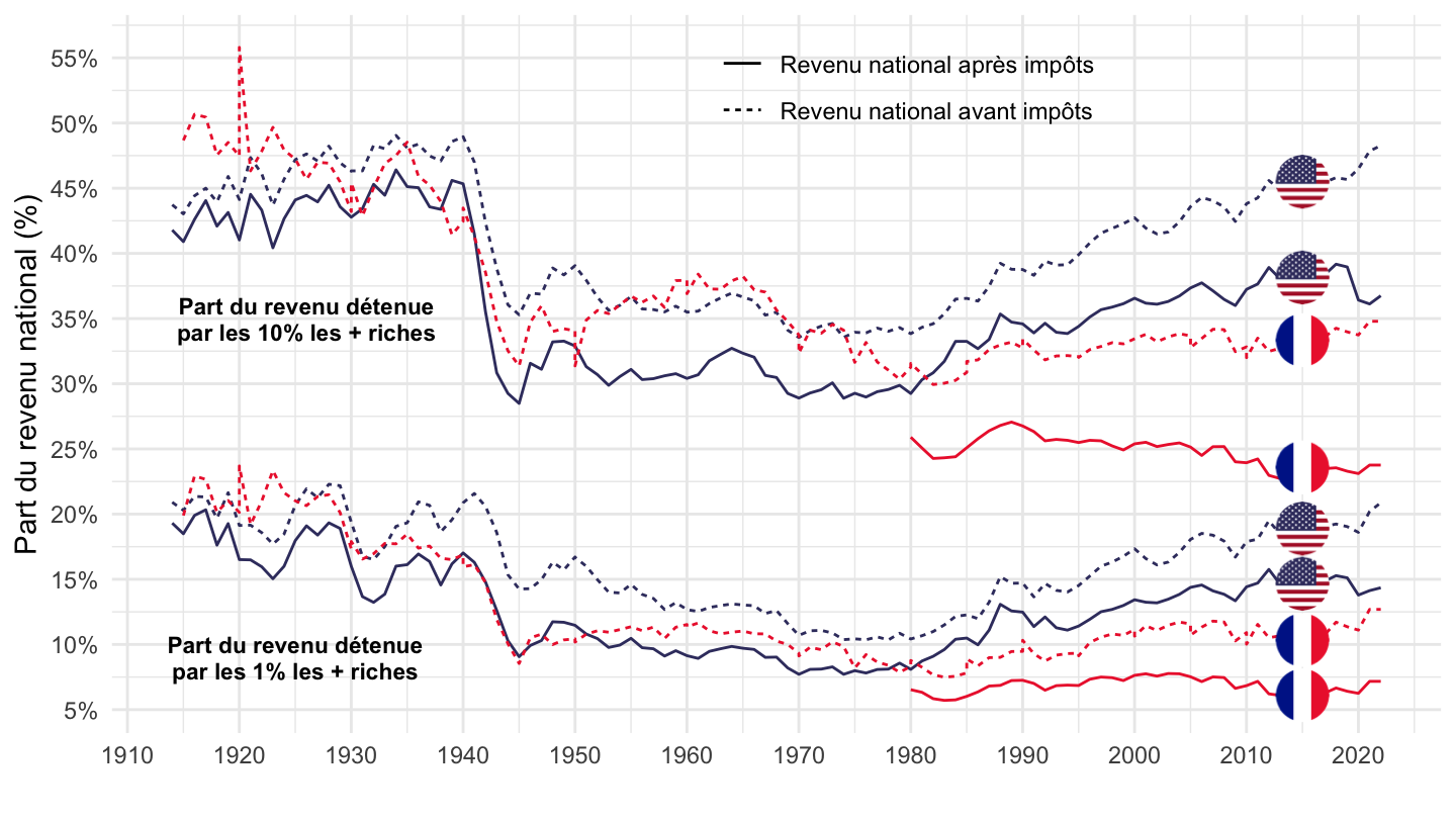
WID_data_DE %>%
  bind_rows(WID_data_FR) %>%
  bind_rows(WID_data_US) %>%
  mutate(name = substr(variable, 2, 6),
         type = substr(variable, 1, 1)) %>%
  filter(name %in% c("ptinc", "diinc"),
         type == "s",
         pop == "j",
         percentile %in% c("p99p100", "p90p100"),
         country %in% c("FR", "DE")) %>%
  year_to_date2() %>%
  filter(date >= as.Date("1914-01-01")) %>%
  left_join(country, by = "country") %>%
  left_join(name, by = "name") %>%
  rename(Location = Country) %>%
  left_join(colors, by = c("Location" = "country")) %>%
  ggplot + geom_line(aes(x = date, y = value, color = color, linetype = shortname, linetype2 = percentile)) +
  scale_color_identity() + ylab("Part du revenu national (%)") + xlab("") + theme_minimal() +
  add_8flags +
  scale_y_continuous(breaks = 0.01*seq(0, 100, 5),
                     labels = scales::percent_format(accuracy = 1)) +
  scale_x_date(breaks = seq(1800, 2025, 10) %>% paste0("-01-01") %>% as.Date,
               labels = date_format("%Y")) +
  theme(legend.position = c(0.6, 0.9),
        legend.title = element_blank()) +
 annotate(geom="text", x = as.Date("1925-01-01"), y = 0.08, label = "par les 1% les + riches", size=3, fontface="bold") +
 annotate(geom="text", x = as.Date("1925-01-01"), y = 0.10, label = "Part du revenu détenue", size=3, fontface="bold") +
 annotate(geom="text", x = as.Date("1926-01-01"), y = 0.34, label = "par les 10% les + riches", size=3, fontface="bold") +
 annotate(geom="text", x = as.Date("1926-01-01"), y = 0.36, label = "Part du revenu détenue", size=3, fontface="bold")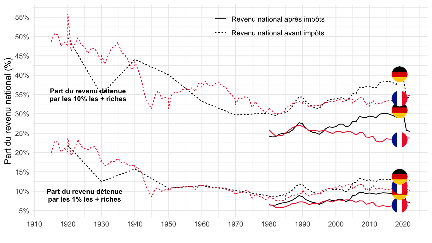
WID_data_DE %>%
  bind_rows(WID_data_FR) %>%
  bind_rows(WID_data_US) %>%
  mutate(name = substr(variable, 2, 6),
         type = substr(variable, 1, 1)) %>%
  filter(name %in% c("ptinc", "diinc"),
         type == "s",
         pop == "j",
         percentile %in% c("p99p100", "p90p100"),
         country %in% c("FR", "DE")) %>%
  year_to_date2() %>%
  filter(date >= as.Date("1999-01-01")) %>%
  left_join(country, by = "country") %>%
  left_join(name, by = "name") %>%
  rename(Location = Country) %>%
  left_join(colors, by = c("Location" = "country")) %>%
  ggplot + geom_line(aes(x = date, y = value, color = color, linetype = shortname, linetype2 = percentile)) +
  scale_color_identity() + ylab("Part du revenu national (%)") + xlab("") + theme_minimal() +
  add_8flags +
  scale_y_continuous(breaks = 0.01*seq(0, 100, 5),
                     labels = scales::percent_format(accuracy = 1)) +
  scale_x_date(breaks = c(seq(1999, 2025, 5), seq(1997, 2025, 5)) %>% paste0("-01-01") %>% as.Date,
               labels = date_format("%Y")) +
  theme(legend.position = c(0.6, 0.9),
        legend.title = element_blank()) +
 annotate(geom="text", x = as.Date("2004-01-01"), y = 0.16, label = "par les 1% les + riches", size=3, fontface="bold") +
 annotate(geom="text", x = as.Date("2004-01-01"), y = 0.18, label = "Part du revenu détenue", size=3, fontface="bold") +
 annotate(geom="text", x = as.Date("2004-01-01"), y = 0.38, label = "par les 10% les + riches", size=3, fontface="bold") +
 annotate(geom="text", x = as.Date("2004-01-01"), y = 0.40, label = "Part du revenu détenue", size=3, fontface="bold")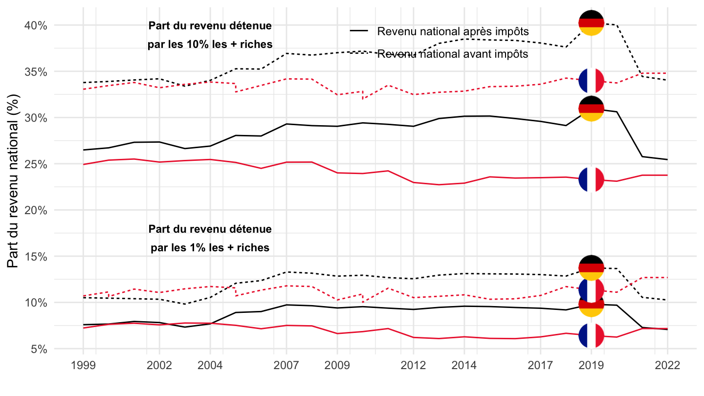
WID_data_DE %>%
  bind_rows(WID_data_FR) %>%
  bind_rows(WID_data_US) %>%
  mutate(name = substr(variable, 2, 6),
         type = substr(variable, 1, 1)) %>%
  filter(name %in% c("ptinc", "diinc"),
         type == "s",
         pop == "j",
         percentile %in% c("p99p100", "p90p100"),
         country %in% c("US", "DE")) %>%
  year_to_date2() %>%
  filter(date >= as.Date("1914-01-01")) %>%
  left_join(country, by = "country") %>%
  rename(Location = Country) %>%
  left_join(colors, by = c("Location" = "country")) %>%
  left_join(name, by = "name") %>%
  mutate(color = ifelse(country == "US", color2, color)) %>%
  ggplot + geom_line(aes(x = date, y = value, color = color, linetype = shortname, linetype2 = percentile)) +
  scale_color_identity() + ylab("Part du revenu national (%)") + xlab("") + theme_minimal() +
  add_8flags +
  scale_y_continuous(breaks = 0.01*seq(0, 100, 5),
                     labels = scales::percent_format(accuracy = 1)) +
  scale_x_date(breaks = seq(1800, 2025, 10) %>% paste0("-01-01") %>% as.Date,
               labels = date_format("%Y")) +
  theme(legend.position = c(0.6, 0.9),
        legend.title = element_blank()) +
 annotate(geom="text", x = as.Date("1925-01-01"), y = 0.08, label = "par les 1% les + riches", size=3, fontface="bold") +
 annotate(geom="text", x = as.Date("1925-01-01"), y = 0.10, label = "Part du revenu détenue", size=3, fontface="bold") +
 annotate(geom="text", x = as.Date("1926-01-01"), y = 0.34, label = "par les 10% les + riches", size=3, fontface="bold") +
 annotate(geom="text", x = as.Date("1926-01-01"), y = 0.36, label = "Part du revenu détenue", size=3, fontface="bold")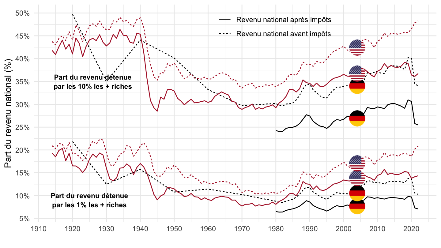
WID_Data_29122021 %>%
  mutate(date = paste0(year, "-01-01") %>% as.Date) %>%
  filter(date >= as.Date("1914-01-01")) %>%
  mutate(Location = ifelse(Location == "USA", "United States", Location),
         pre_post = case_when(grepl("Post-tax", Variable) ~ "Après redistribution",
                              grepl("Pre-tax", Variable) ~ "Avant redistribution"),
         top = case_when(grepl("Top 1%", Variable) ~ "Top 1%",
                              grepl("Top 10%", Variable) ~ "Top 10%")) %>%
  left_join(colors, by = c("Location" = "country")) %>%

  ggplot + geom_line(aes(x = date, y = value, color = color, linetype = pre_post, linetype2 = top)) +
  scale_color_identity() + ylab("Part du revenu national (%)") + xlab("") + theme_minimal() +
  add_8flags +
  scale_y_continuous(breaks = 0.01*seq(0, 100, 5),
                     labels = scales::percent_format(accuracy = 1)) +
  scale_x_date(breaks = seq(1800, 2025, 10) %>% paste0("-01-01") %>% as.Date,
               labels = date_format("%Y")) +
  theme(legend.position = c(0.6, 0.9),
        legend.title = element_blank()) +
 annotate(geom="text", x = as.Date("1925-01-01"), y = 0.08, label = "par les 1% les + riches", size=3, fontface="bold") +
 annotate(geom="text", x = as.Date("1925-01-01"), y = 0.10, label = "Part du revenu détenue", size=3, fontface="bold") +
 annotate(geom="text", x = as.Date("1926-01-01"), y = 0.34, label = "par les 10% les + riches", size=3, fontface="bold") +
 annotate(geom="text", x = as.Date("1926-01-01"), y = 0.36, label = "Part du revenu détenue", size=3, fontface="bold")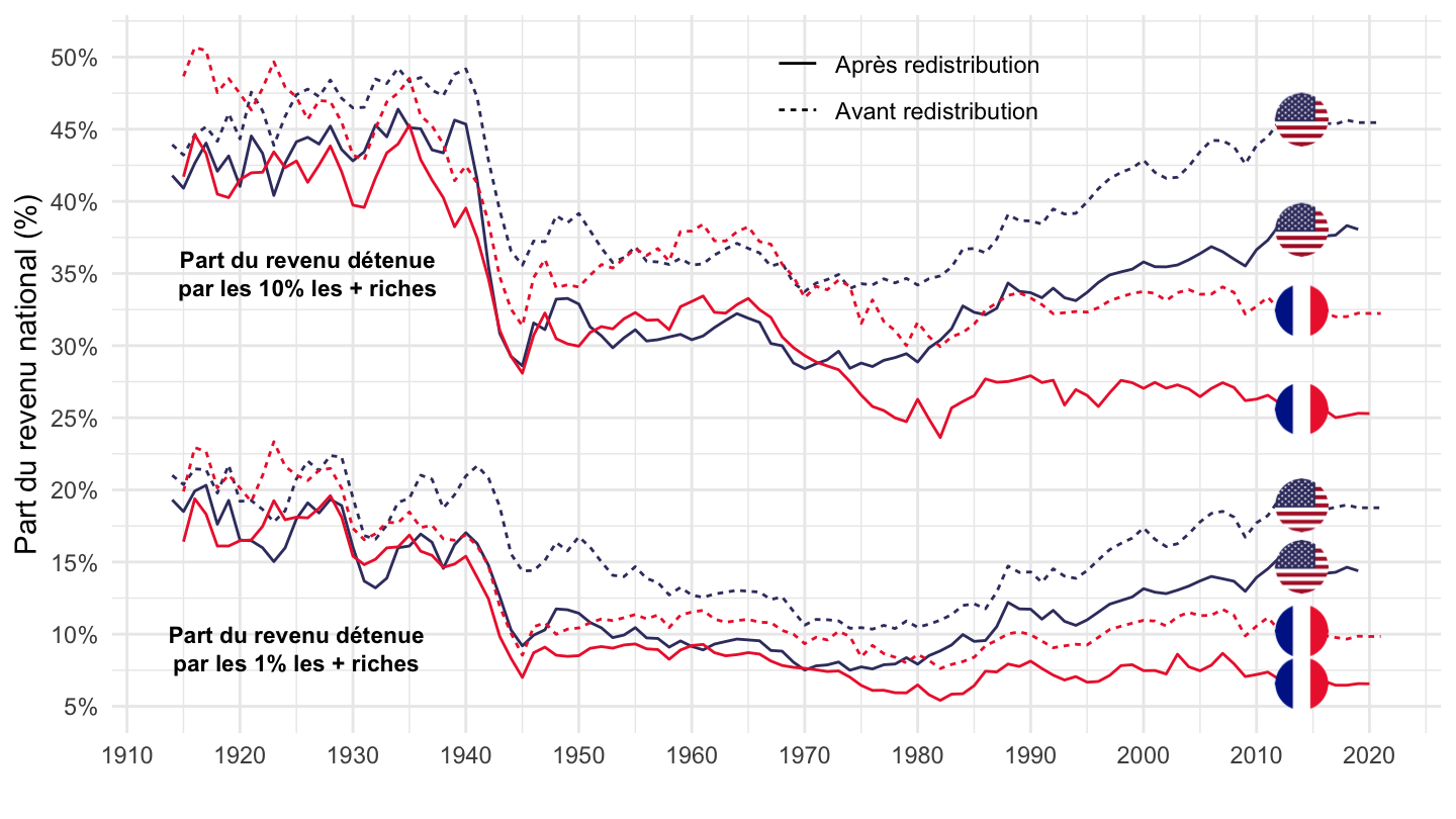
WID_Data_29122021 %>%
  mutate(date = paste0(year, "-01-01") %>% as.Date) %>%
  filter(date >= as.Date("1914-01-01")) %>%
  mutate(Location = ifelse(Location == "USA", "United States", Location),
         pre_post = case_when(grepl("Post-tax", Variable) ~ "Après redistribution",
                              grepl("Pre-tax", Variable) ~ "Avant redistribution"),
         top = case_when(grepl("Top 1%", Variable) ~ "Top 1%",
                              grepl("Top 10%", Variable) ~ "Top 10%")) %>%
  left_join(colors, by = c("Location" = "country")) %>%

  ggplot + geom_line(aes(x = date, y = value, color = color, linetype = pre_post, linetype2 = top)) +
  scale_color_identity() + ylab("Part du revenu national (%)") + xlab("") + theme_minimal() +
  add_8flags +
  scale_y_continuous(breaks = 0.01*seq(0, 100, 5),
                     labels = scales::percent_format(accuracy = 1),
                     limits = c(0, 0.52)) +
  scale_x_date(breaks = seq(1800, 2025, 10) %>% paste0("-01-01") %>% as.Date,
               labels = date_format("%Y")) +
  theme(legend.position = c(0.6, 0.9),
        legend.title = element_blank()) +
 annotate(geom="text", x = as.Date("1925-01-01"), y = 0.08, label = "par les 1% les + riches", size=3, fontface="bold") +
 annotate(geom="text", x = as.Date("1925-01-01"), y = 0.10, label = "Part du revenu détenue", size=3, fontface="bold") +
 annotate(geom="text", x = as.Date("1926-01-01"), y = 0.34, label = "par les 10% les + riches", size=3, fontface="bold") +
 annotate(geom="text", x = as.Date("1926-01-01"), y = 0.36, label = "Part du revenu détenue", size=3, fontface="bold")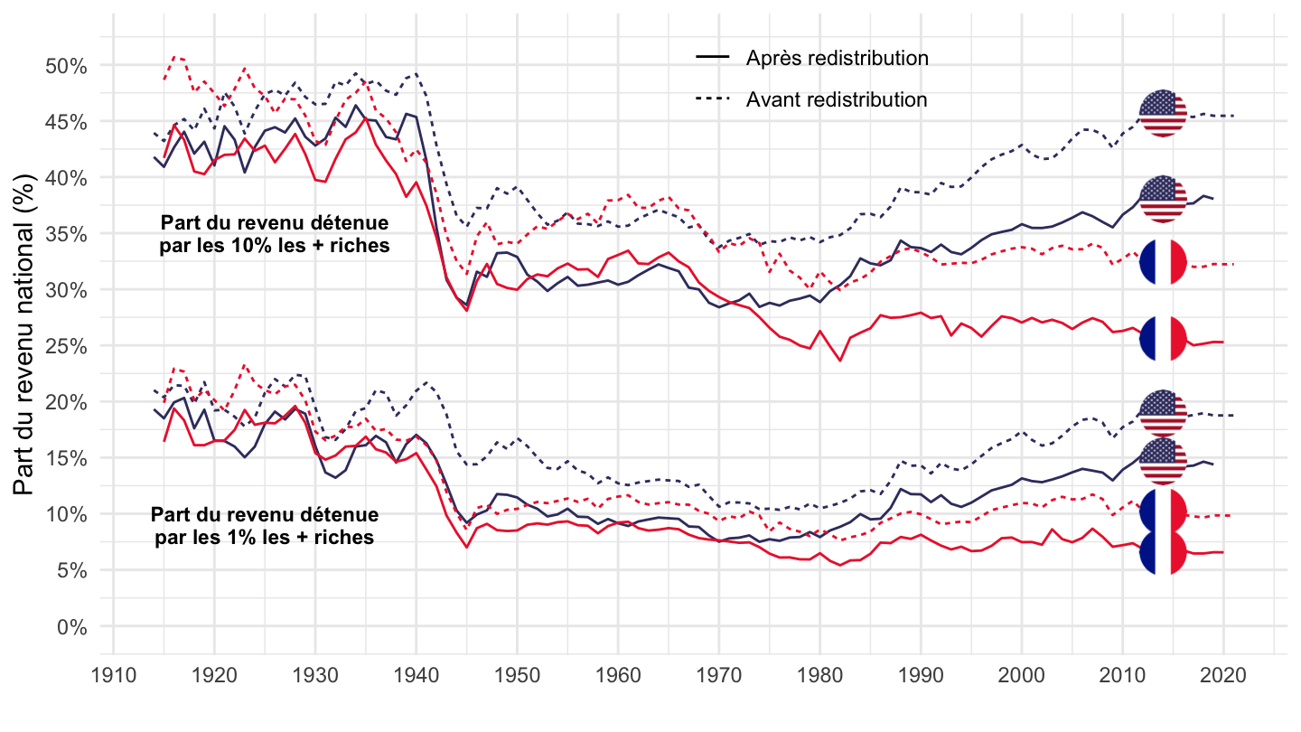
WID_Data_29122021 %>%
  mutate(date = paste0(year, "-01-01") %>% as.Date) %>%
  filter(date >= as.Date("1914-01-01")) %>%
  mutate(Location = ifelse(Location == "USA", "United States", Location),
         pre_post = case_when(grepl("Post-tax", Variable) ~ "Après redistribution",
                              grepl("Pre-tax", Variable) ~ "Avant redistribution"),
         top = case_when(grepl("Top 1%", Variable) ~ "Top 1%",
                              grepl("Top 10%", Variable) ~ "Top 10%")) %>%
  left_join(colors, by = c("Location" = "country")) %>%
  filter(date>= as.Date("1999-01-01")) %>%
  ggplot + geom_line(aes(x = date, y = value, color = color, linetype = pre_post, linetype2 = top)) +
  scale_color_identity() + ylab("Part du revenu national (%)") + xlab("") + theme_minimal() +
  add_8flags +
  scale_y_continuous(breaks = 0.01*seq(0, 100, 5),
                     labels = scales::percent_format(accuracy = 1),
                     limits = c(0, 0.52)) +
  scale_x_date(breaks = seq(1800, 2025, 10) %>% paste0("-01-01") %>% as.Date,
               labels = date_format("%Y")) +
  theme(legend.position = c(0.6, 0.9),
        legend.title = element_blank()) +
 annotate(geom="text", x = as.Date("2005-01-01"), y = 0.08, label = "par les 1% les + riches", size=3, fontface="bold") +
 annotate(geom="text", x = as.Date("2005-01-01"), y = 0.10, label = "Part du revenu détenue", size=3, fontface="bold") +
 annotate(geom="text", x = as.Date("2005-01-01"), y = 0.34, label = "par les 10% les + riches", size=3, fontface="bold") +
 annotate(geom="text", x = as.Date("2005-01-01"), y = 0.36, label = "Part du revenu détenue", size=3, fontface="bold")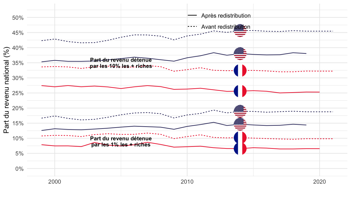
WID_Data_29122021 %>%
  mutate(date = paste0(year, "-01-01") %>% as.Date) %>%
  filter(date >= as.Date("1914-01-01")) %>%
  mutate(Location = ifelse(Location == "USA", "United States", Location),
         pre_post = case_when(grepl("Post-tax", Variable) ~ "Après redistribution",
                              grepl("Pre-tax", Variable) ~ "Avant redistribution"),
         top = case_when(grepl("Top 1%", Variable) ~ "Top 1%",
                              grepl("Top 10%", Variable) ~ "Top 10%")) %>%
  left_join(colors, by = c("Location" = "country")) %>%
  filter(grepl("Pre-tax", Variable)) %>%

  ggplot + geom_line(aes(x = date, y = value, color = color, linetype2 = top)) +
  scale_color_identity() + ylab("Part du revenu national, avant redistribution (%)") + xlab("") + theme_minimal() +
  add_4flags +
  scale_y_continuous(breaks = 0.01*seq(0, 100, 5),
                     labels = scales::percent_format(accuracy = 1)) +
  scale_x_date(breaks = seq(1800, 2025, 10) %>% paste0("-01-01") %>% as.Date,
               labels = date_format("%Y")) +
  theme(legend.position = c(0.6, 0.9),
        legend.title = element_blank()) +
 annotate(geom="text", x = as.Date("1925-01-01"), y = 0.08, label = "par les 1% les + riches", size=3, fontface="bold") +
 annotate(geom="text", x = as.Date("1925-01-01"), y = 0.10, label = "Part du revenu détenue", size=3, fontface="bold") +
 annotate(geom="text", x = as.Date("1926-01-01"), y = 0.34, label = "par les 10% les + riches", size=3, fontface="bold") +
 annotate(geom="text", x = as.Date("1926-01-01"), y = 0.36, label = "Part du revenu détenue", size=3, fontface="bold")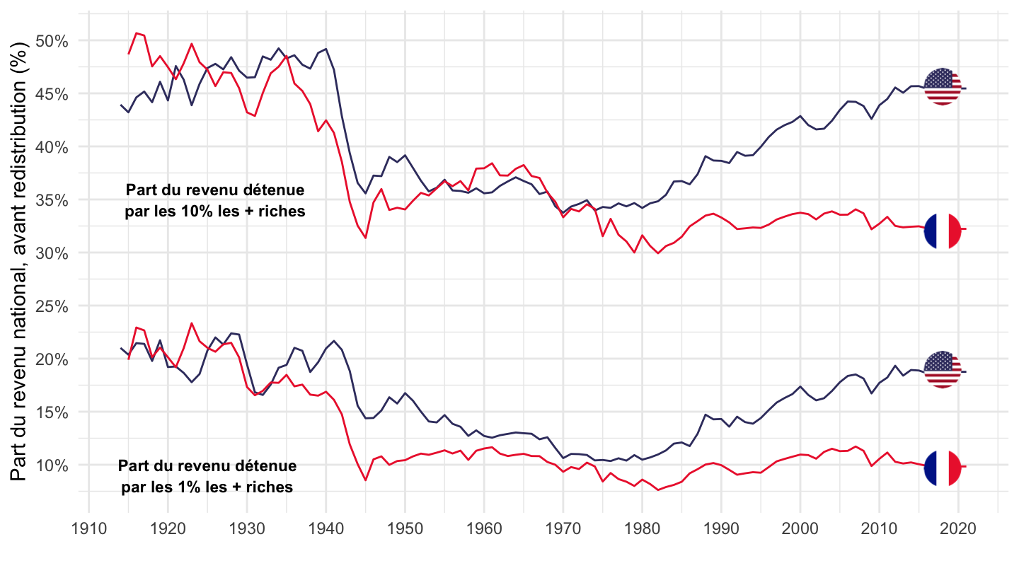
WID_Data_29122021 %>%
  mutate(date = paste0(year, "-01-01") %>% as.Date) %>%
  filter(date >= as.Date("1914-01-01")) %>%
  mutate(Location = ifelse(Location == "USA", "United States", Location),
         pre_post = case_when(grepl("Post-tax", Variable) ~ "Après redistribution",
                              grepl("Pre-tax", Variable) ~ "Avant redistribution"),
         top = case_when(grepl("Top 1%", Variable) ~ "Top 1%",
                              grepl("Top 10%", Variable) ~ "Top 10%")) %>%
  left_join(colors, by = c("Location" = "country")) %>%
  filter(grepl("Pre-tax", Variable)) %>%

  ggplot + geom_line(aes(x = date, y = value, color = color, linetype2 = top)) +
  scale_color_identity() + ylab("Part du revenu national, avant redistribution (%)") + xlab("") + theme_minimal() +
  add_4flags +
  scale_y_continuous(breaks = 0.01*seq(0, 100, 5),
                     labels = scales::percent_format(accuracy = 1),
                     limits = c(0, 0.52)) +
  scale_x_date(breaks = seq(1800, 2025, 10) %>% paste0("-01-01") %>% as.Date,
               labels = date_format("%Y")) +
  theme(legend.position = c(0.6, 0.9),
        legend.title = element_blank()) +
 annotate(geom="text", x = as.Date("1925-01-01"), y = 0.08, label = "par les 1% les + riches", size=3, fontface="bold") +
 annotate(geom="text", x = as.Date("1925-01-01"), y = 0.10, label = "Part du revenu détenue", size=3, fontface="bold") +
 annotate(geom="text", x = as.Date("1926-01-01"), y = 0.34, label = "par les 10% les + riches", size=3, fontface="bold") +
 annotate(geom="text", x = as.Date("1926-01-01"), y = 0.36, label = "Part du revenu détenue", size=3, fontface="bold")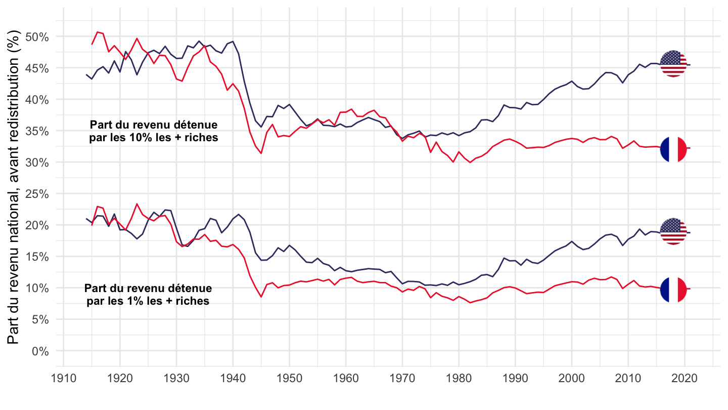
WID_Data_29122021 %>%
  mutate(date = paste0(year, "-01-01") %>% as.Date) %>%
  filter(date >= as.Date("1914-01-01")) %>%
  mutate(Location = ifelse(Location == "USA", "United States", Location),
         pre_post = case_when(grepl("Post-tax", Variable) ~ "Après redistribution",
                              grepl("Pre-tax", Variable) ~ "Avant redistribution"),
         top = case_when(grepl("Top 1%", Variable) ~ "Top 1%",
                              grepl("Top 10%", Variable) ~ "Top 10%")) %>%
  left_join(colors, by = c("Location" = "country")) %>%
  filter(grepl("Post-tax", Variable)) %>%

  ggplot + geom_line(aes(x = date, y = value, color = color, linetype2 = top)) +
  scale_color_identity() + ylab("Part du revenu national, après redistribution (%)") + xlab("") + theme_minimal() +
  add_4flags +
  scale_y_continuous(breaks = 0.01*seq(0, 100, 5),
                     labels = scales::percent_format(accuracy = 1)) +
  scale_x_date(breaks = seq(1800, 2025, 10) %>% paste0("-01-01") %>% as.Date,
               labels = date_format("%Y")) +
  theme(legend.position = c(0.6, 0.9),
        legend.title = element_blank()) +
 annotate(geom="text", x = as.Date("1925-01-01"), y = 0.08, label = "par les 1% les + riches", size=3, fontface="bold") +
 annotate(geom="text", x = as.Date("1925-01-01"), y = 0.10, label = "Part du revenu détenue", size=3, fontface="bold") +
 annotate(geom="text", x = as.Date("1926-01-01"), y = 0.34, label = "par les 10% les + riches", size=3, fontface="bold") +
 annotate(geom="text", x = as.Date("1926-01-01"), y = 0.36, label = "Part du revenu détenue", size=3, fontface="bold")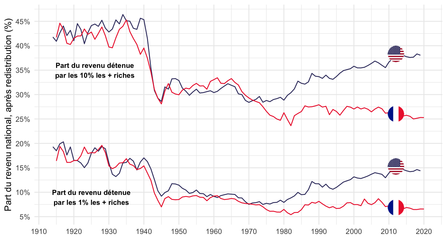
WID_Data_29122021 %>%
  mutate(date = paste0(year, "-01-01") %>% as.Date) %>%
  filter(date >= as.Date("1914-01-01")) %>%
  mutate(Location = ifelse(Location == "USA", "United States", Location),
         pre_post = case_when(grepl("Post-tax", Variable) ~ "Après redistribution",
                              grepl("Pre-tax", Variable) ~ "Avant redistribution"),
         top = case_when(grepl("Top 1%", Variable) ~ "Top 1%",
                              grepl("Top 10%", Variable) ~ "Top 10%")) %>%
  left_join(colors, by = c("Location" = "country")) %>%
  filter(grepl("Post-tax", Variable)) %>%

  ggplot + geom_line(aes(x = date, y = value, color = color, linetype2 = top)) +
  scale_color_identity() + ylab("Part du revenu national, après redistribution (%)") + xlab("") + theme_minimal() +
  add_4flags +
  scale_y_continuous(breaks = 0.01*seq(0, 100, 5),
                     labels = scales::percent_format(accuracy = 1),
                     limits = c(0, 0.47)) +
  scale_x_date(breaks = seq(1800, 2025, 10) %>% paste0("-01-01") %>% as.Date,
               labels = date_format("%Y")) +
  theme(legend.position = c(0.6, 0.9),
        legend.title = element_blank()) +
 annotate(geom="text", x = as.Date("1925-01-01"), y = 0.08, label = "par les 1% les + riches", size=3, fontface="bold") +
 annotate(geom="text", x = as.Date("1925-01-01"), y = 0.10, label = "Part du revenu détenue", size=3, fontface="bold") +
 annotate(geom="text", x = as.Date("1926-01-01"), y = 0.34, label = "par les 10% les + riches", size=3, fontface="bold") +
 annotate(geom="text", x = as.Date("1926-01-01"), y = 0.36, label = "Part du revenu détenue", size=3, fontface="bold")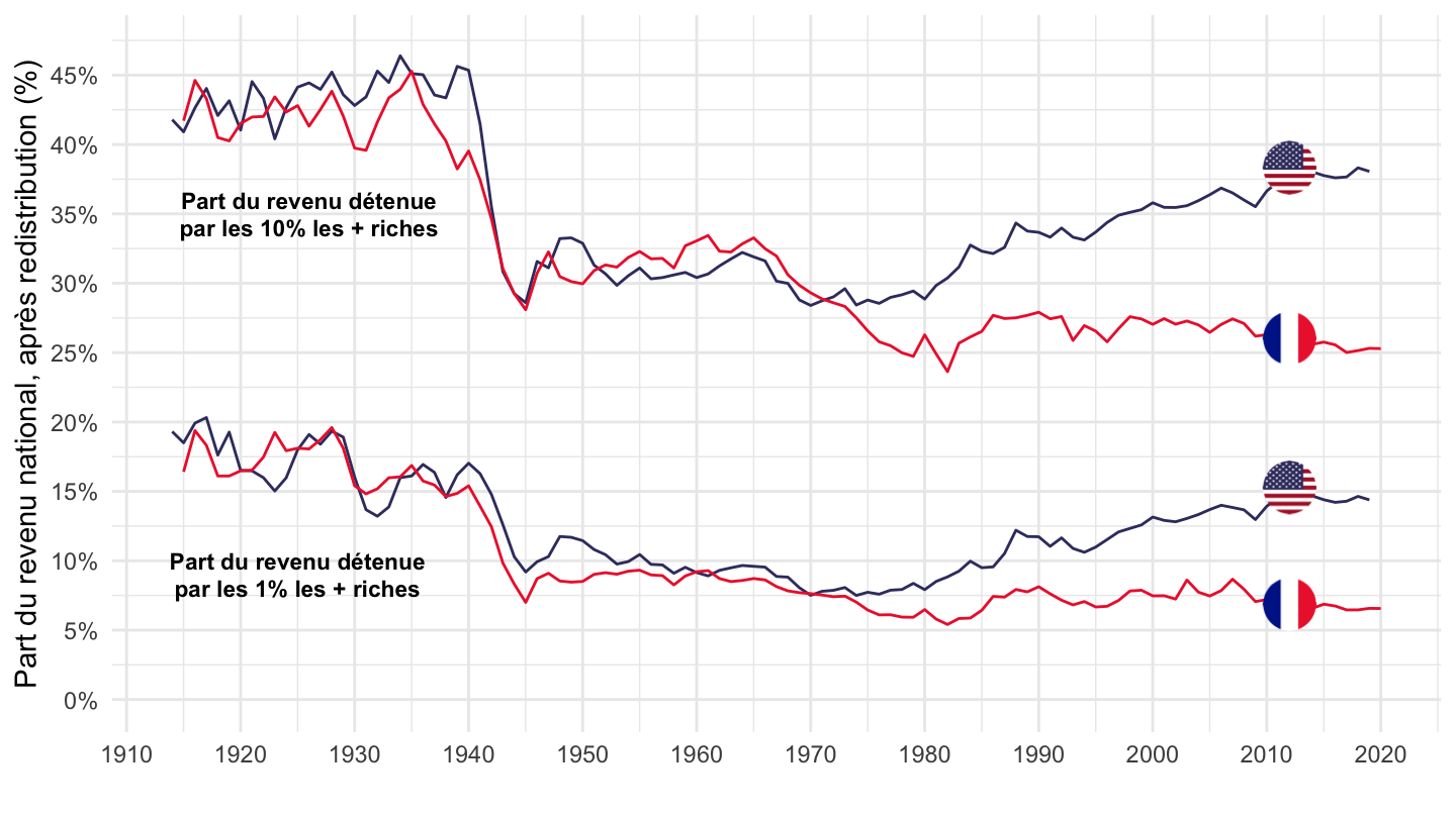
WID_data_DE %>%
  bind_rows(WID_data_FR) %>%
  bind_rows(WID_data_US) %>%
  mutate(name = substr(variable, 2, 6),
         type = substr(variable, 1, 1)) %>%
  filter(name %in% c("hweal"),
         type == "s",
         pop == "j",
         percentile %in% c("p99p100", "p90p100"),
         country %in% c("US", "FR")) %>%
  year_to_date2() %>%
  filter(date >= as.Date("1914-01-01")) %>%
  left_join(country, by = "country") %>%
  rename(Location = Country) %>%
  left_join(colors, by = c("Location" = "country")) %>%
  left_join(name, by = "name") %>%
  ggplot + geom_line(aes(x = date, y = value, color = color, linetype = percentile)) +
  scale_color_identity() + ylab("Part de la richesse (%)") + xlab("") + theme_minimal() +
  add_4flags +
  scale_y_continuous(breaks = 0.01*seq(0, 100, 5),
                     labels = scales::percent_format(accuracy = 1)) +
  scale_x_date(breaks = seq(1800, 2025, 10) %>% paste0("-01-01") %>% as.Date,
               labels = date_format("%Y")) +
  theme(legend.position = c(0.6, 0.9),
        legend.title = element_blank()) +
 annotate(geom="text", x = as.Date("1925-01-01"), y = 0.25, label = "par les 1% les + riches", size=3, fontface="bold") +
 annotate(geom="text", x = as.Date("1925-01-01"), y = 0.27, label = "Part de la richesse détenue", size=3, fontface="bold") +
 annotate(geom="text", x = as.Date("1926-01-01"), y = 0.65, label = "par les 10% les + riches", size=3, fontface="bold") +
 annotate(geom="text", x = as.Date("1926-01-01"), y = 0.67, label = "Part de la richesse détenue", size=3, fontface="bold")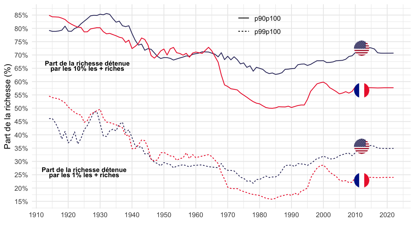
WID_data_IT %>%
  bind_rows(WID_data_FR) %>%
  bind_rows(WID_data_US) %>%
  mutate(name = substr(variable, 2, 6),
         type = substr(variable, 1, 1)) %>%
  filter(name %in% c("hweal"),
         type == "s",
         pop == "j",
         percentile %in% c("p99p100", "p90p100"),
         country %in% c("US", "FR", "IT")) %>%
  year_to_date2() %>%
  filter(date >= as.Date("1914-01-01")) %>%
  left_join(country, by = "country") %>%
  rename(Location = Country) %>%
  left_join(colors, by = c("Location" = "country")) %>%
  left_join(name, by = "name") %>%
  ggplot + geom_line(aes(x = date, y = value, color = color, linetype = percentile)) +
  scale_color_identity() + ylab("Part de la richesse (%)") + xlab("") + theme_minimal() +
  add_4flags +
  scale_y_continuous(breaks = 0.01*seq(0, 100, 5),
                     labels = scales::percent_format(accuracy = 1)) +
  scale_x_date(breaks = seq(1800, 2025, 10) %>% paste0("-01-01") %>% as.Date,
               labels = date_format("%Y")) +
  theme(legend.position = c(0.6, 0.9),
        legend.title = element_blank()) +
 annotate(geom="text", x = as.Date("1925-01-01"), y = 0.25, label = "par les 1% les + riches", size=3, fontface="bold") +
 annotate(geom="text", x = as.Date("1925-01-01"), y = 0.27, label = "Part de la richesse détenue", size=3, fontface="bold") +
 annotate(geom="text", x = as.Date("1926-01-01"), y = 0.65, label = "par les 10% les + riches", size=3, fontface="bold") +
 annotate(geom="text", x = as.Date("1926-01-01"), y = 0.67, label = "Part de la richesse détenue", size=3, fontface="bold")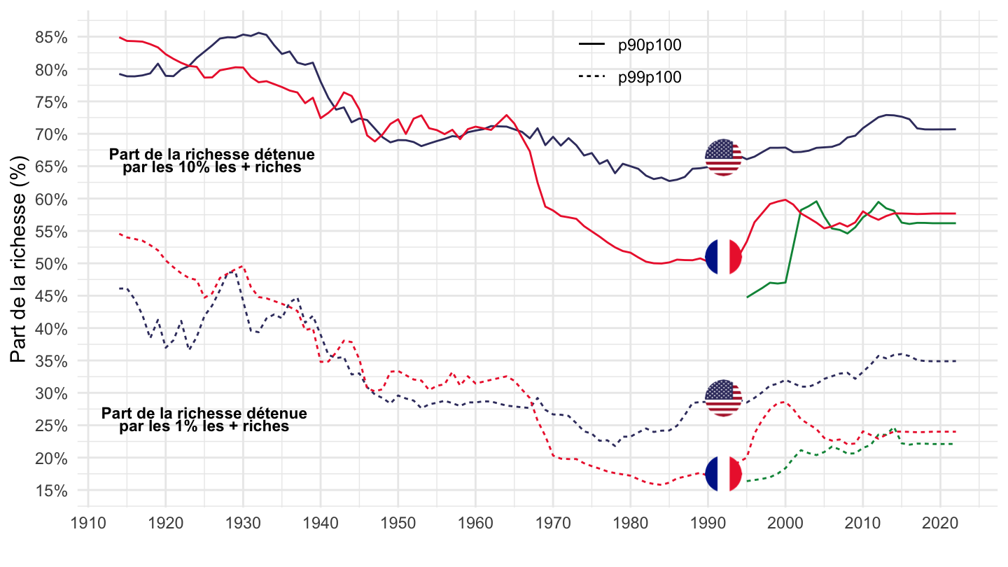
WID_data_SE %>%
  bind_rows(WID_data_FR) %>%
  bind_rows(WID_data_US) %>%
  mutate(name = substr(variable, 2, 6),
         type = substr(variable, 1, 1)) %>%
  filter(name %in% c("hweal"),
         type == "s",
         pop == "j",
         percentile %in% c("p99p100", "p90p100"),
         country %in% c("US", "FR", "SE")) %>%
  year_to_date2() %>%
  left_join(country, by = "country") %>%
  rename(Location = Country) %>%
  left_join(colors, by = c("Location" = "country")) %>%
  left_join(name, by = "name") %>%
  ggplot + geom_line(aes(x = date, y = value, color = color, linetype = percentile)) +
  scale_color_identity() + ylab("Part de la richesse (%)") + xlab("") + theme_minimal() +
  add_6flags +
  scale_y_continuous(breaks = 0.01*seq(0, 100, 5),
                     labels = scales::percent_format(accuracy = 1)) +
  scale_x_date(breaks = seq(1800, 2025, 20) %>% paste0("-01-01") %>% as.Date,
               labels = date_format("%Y")) +
  theme(legend.position = c(0.6, 0.9),
        legend.title = element_blank()) +
 annotate(geom="text", x = as.Date("1925-01-01"), y = 0.25, label = "par les 1% les + riches", size=3, fontface="bold") +
 annotate(geom="text", x = as.Date("1925-01-01"), y = 0.27, label = "Part de la richesse détenue", size=3, fontface="bold") +
 annotate(geom="text", x = as.Date("1926-01-01"), y = 0.65, label = "par les 10% les + riches", size=3, fontface="bold") +
 annotate(geom="text", x = as.Date("1926-01-01"), y = 0.67, label = "Part de la richesse détenue", size=3, fontface="bold")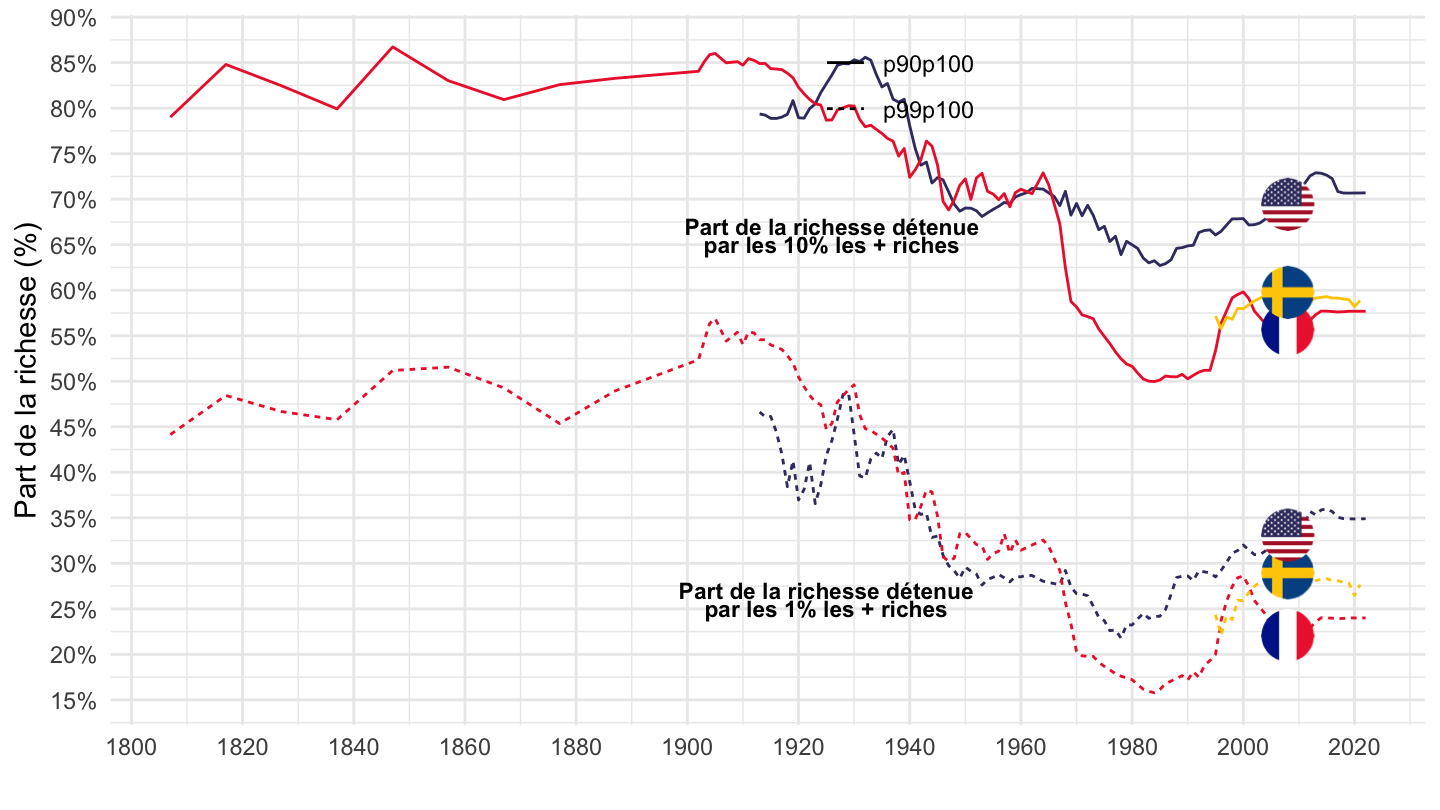
WID_data_SE %>%
  bind_rows(WID_data_FR) %>%
  bind_rows(WID_data_US) %>%
  mutate(name = substr(variable, 2, 6),
         type = substr(variable, 1, 1)) %>%
  filter(name %in% c("hweal"),
         type == "s",
         pop == "j",
         percentile %in% c("p99p100", "p90p100"),
         country %in% c("US", "FR", "SE")) %>%
  year_to_date2() %>%
  filter(date >= as.Date("1914-01-01")) %>%
  left_join(country, by = "country") %>%
  rename(Location = Country) %>%
  left_join(colors, by = c("Location" = "country")) %>%
  left_join(name, by = "name") %>%
  ggplot + geom_line(aes(x = date, y = value, color = color, linetype = percentile)) +
  scale_color_identity() + ylab("Part de la richesse (%)") + xlab("") + theme_minimal() +
  add_6flags +
  scale_y_continuous(breaks = 0.01*seq(0, 100, 5),
                     labels = scales::percent_format(accuracy = 1)) +
  scale_x_date(breaks = seq(1800, 2025, 10) %>% paste0("-01-01") %>% as.Date,
               labels = date_format("%Y")) +
  theme(legend.position = c(0.6, 0.9),
        legend.title = element_blank()) +
 annotate(geom="text", x = as.Date("1925-01-01"), y = 0.25, label = "par les 1% les + riches", size=3, fontface="bold") +
 annotate(geom="text", x = as.Date("1925-01-01"), y = 0.27, label = "Part de la richesse détenue", size=3, fontface="bold") +
 annotate(geom="text", x = as.Date("1926-01-01"), y = 0.65, label = "par les 10% les + riches", size=3, fontface="bold") +
 annotate(geom="text", x = as.Date("1926-01-01"), y = 0.67, label = "Part de la richesse détenue", size=3, fontface="bold")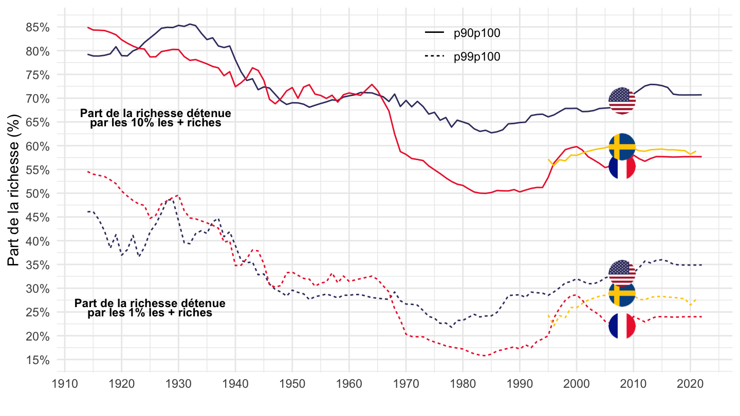
WID_data_SE %>%
  bind_rows(WID_data_FR) %>%
  bind_rows(WID_data_US) %>%
  mutate(name = substr(variable, 2, 6),
         type = substr(variable, 1, 1)) %>%
  filter(name %in% c("hweal"),
         type == "s",
         pop == "j",
         percentile %in% c("p99p100", "p90p100"),
         country %in% c("US", "FR", "SE")) %>%
  year_to_date2() %>%
  filter(date >= as.Date("1995-01-01")) %>%
  left_join(country, by = "country") %>%
  rename(Location = Country) %>%
  left_join(colors, by = c("Location" = "country")) %>%
  left_join(name, by = "name") %>%
  ggplot + geom_line(aes(x = date, y = value, color = color, linetype = percentile)) +
  scale_color_identity() + ylab("Part de la richesse (%)") + xlab("") + theme_minimal() +
  add_6flags +
  scale_y_continuous(breaks = 0.01*seq(0, 100, 5),
                     labels = scales::percent_format(accuracy = 1)) +
  scale_x_date(breaks = seq(1800, 2025, 5) %>% paste0("-01-01") %>% as.Date,
               labels = date_format("%Y")) +
  theme(legend.position = c(0.6, 0.9),
        legend.title = element_blank()) +
 annotate(geom="text", x = as.Date("2000-01-01"), y = 0.25, label = "par les 1% les + riches", size=3, fontface="bold") +
 annotate(geom="text", x = as.Date("2000-01-01"), y = 0.27, label = "Part de la richesse détenue", size=3, fontface="bold") +
 annotate(geom="text", x = as.Date("2001-01-01"), y = 0.65, label = "par les 10% les + riches", size=3, fontface="bold") +
 annotate(geom="text", x = as.Date("2001-01-01"), y = 0.67, label = "Part de la richesse détenue", size=3, fontface="bold")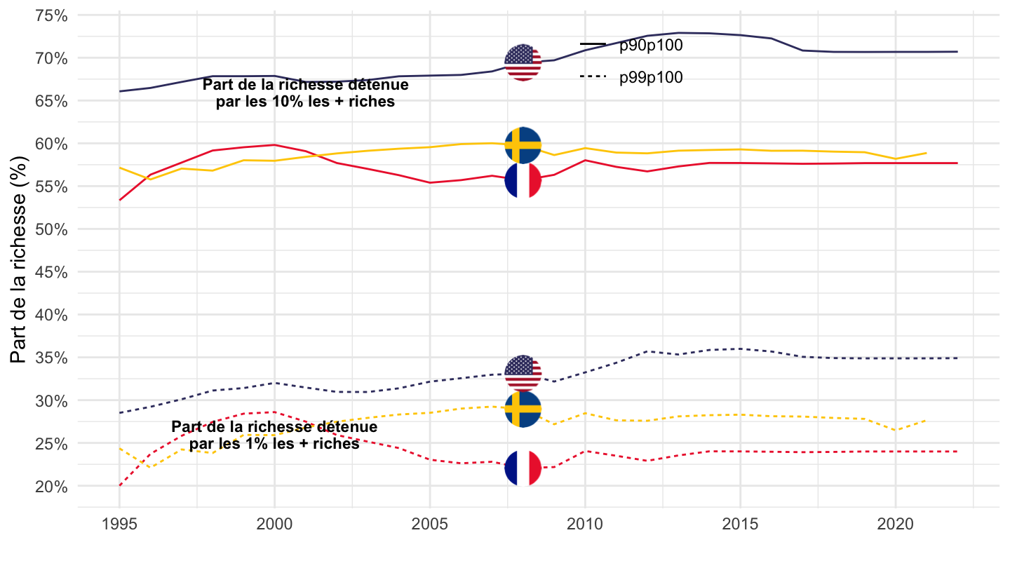
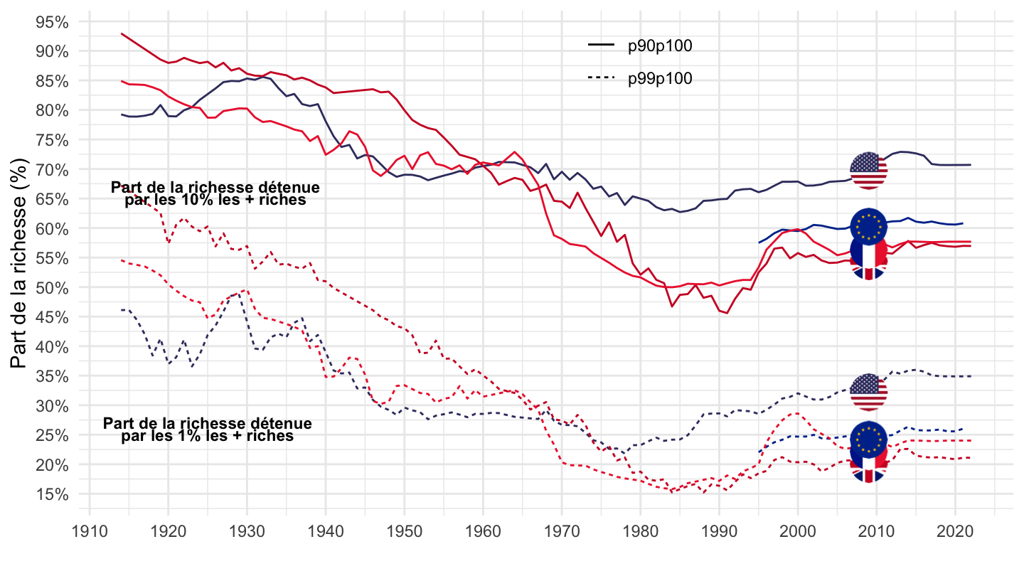
WID_data_GB %>%
  bind_rows(WID_data_FR) %>%
  bind_rows(WID_data_US) %>%
  bind_rows(WID_data_QE) %>%
  mutate(name = substr(variable, 2, 6),
         type = substr(variable, 1, 1)) %>%
  filter(name %in% c("hweal"),
         type == "s",
         pop == "j",
         percentile %in% c("p99p100", "p90p100"),
         country %in% c("US", "FR", "GB", "QE")) %>%
  year_to_date2() %>%
  filter(date >= as.Date("1914-01-01")) %>%
  left_join(country, by = "country") %>%
  rename(Location = Country) %>%
  left_join(colors, by = c("Location" = "country")) %>%
  left_join(name, by = "name") %>%
  ggplot + geom_line(aes(x = date, y = value, color = color, linetype = percentile)) +
  scale_color_identity() + ylab("Part de la richesse (%)") + xlab("") + theme_minimal() +
  add_8flags +
  scale_y_continuous(breaks = 0.01*seq(0, 100, 5),
                     labels = scales::percent_format(accuracy = 1)) +
  scale_x_date(breaks = seq(1800, 2025, 10) %>% paste0("-01-01") %>% as.Date,
               labels = date_format("%Y")) +
  theme(legend.position = c(0.6, 0.9),
        legend.title = element_blank()) +
 annotate(geom="text", x = as.Date("1925-01-01"), y = 0.25, label = "par les 1% les + riches", size=3, fontface="bold") +
 annotate(geom="text", x = as.Date("1925-01-01"), y = 0.27, label = "Part de la richesse détenue", size=3, fontface="bold") +
 annotate(geom="text", x = as.Date("1926-01-01"), y = 0.65, label = "par les 10% les + riches", size=3, fontface="bold") +
 annotate(geom="text", x = as.Date("1926-01-01"), y = 0.67, label = "Part de la richesse détenue", size=3, fontface="bold")