SP.POP.TOTL %>%
right_join(iso2c, by = "iso2c") %>%
filter(iso2c %in% c("1W", "US", "CN", "EU")) %>%
group_by(year) %>%
mutate(value = value/value[iso2c == "1W"]) %>%
year_to_date %>%
filter(!(iso2c == "1W")) %>%
mutate(Iso2c = ifelse(iso2c == "EU", "Europe", Iso2c)) %>%
left_join(colors, by = c("Iso2c" = "country")) %>%
mutate(color = ifelse(iso2c == "US", color2, color)) %>%
ggplot(.) + theme_minimal() + scale_color_identity() +
geom_line(aes(x = date, y = value, color = color)) +
add_3flags +
scale_x_date(breaks = seq(1950, 2100, 5) %>% paste0("-01-01") %>% as.Date,
labels = date_format("%Y")) +
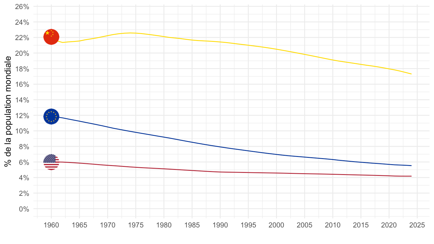
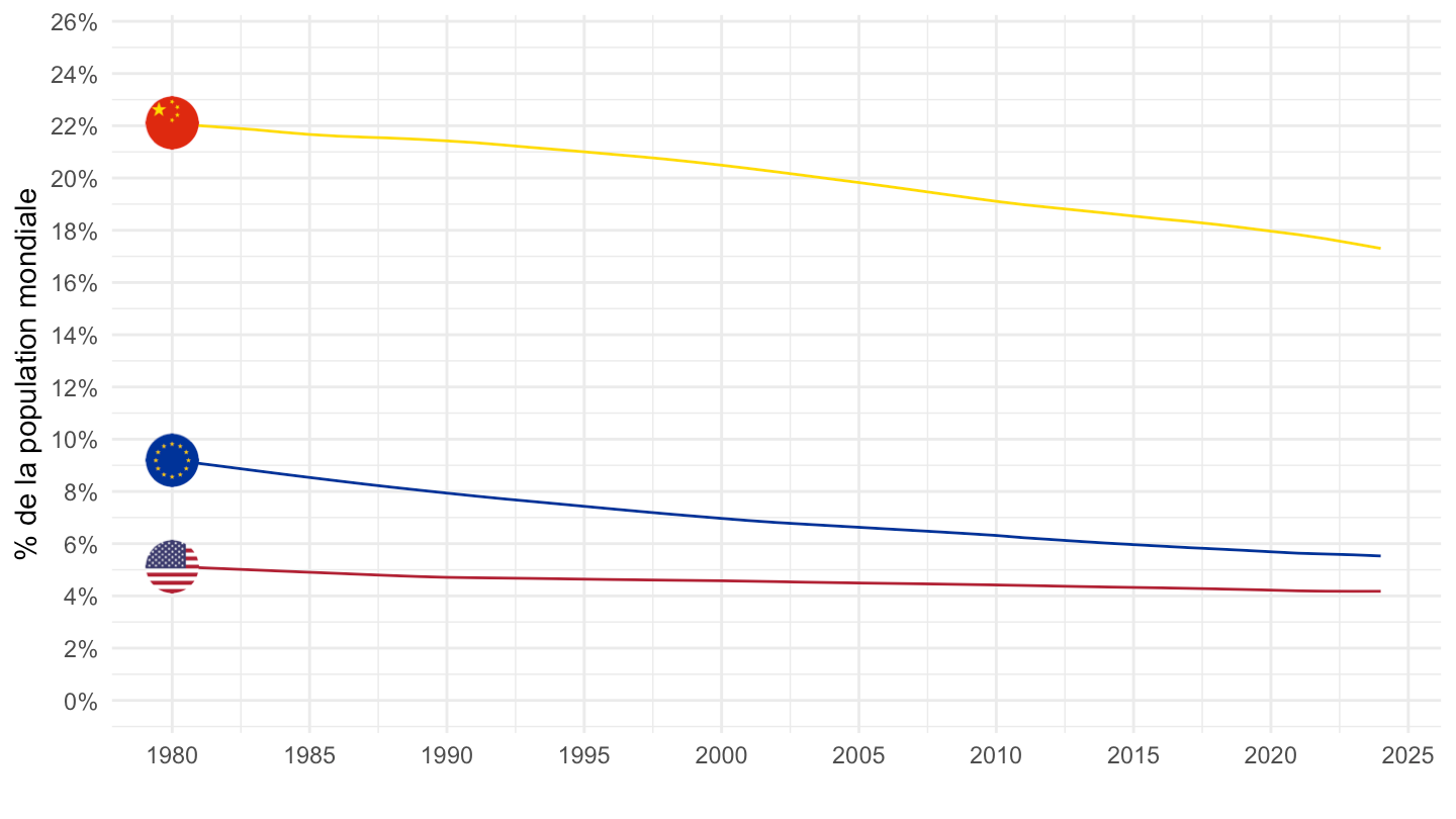
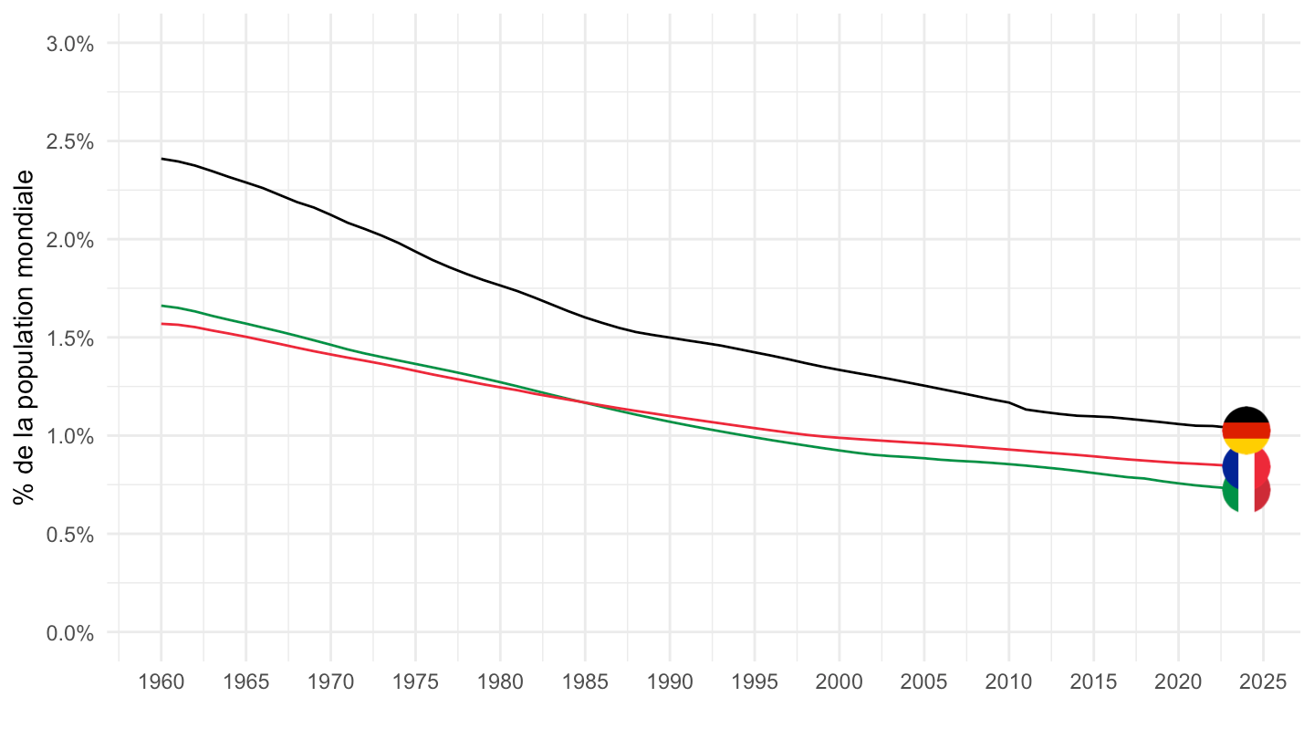
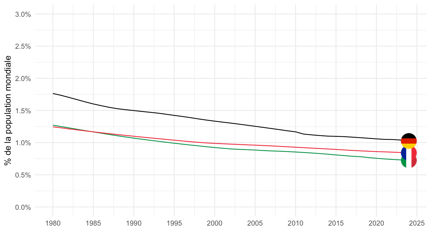
scale_y_continuous(breaks = 0.01*seq(0, 70, 2),
labels = scales::percent_format(accuracy = 1),
limits = 0.01*c(0, 25)) +
xlab("") + ylab("% de la population mondiale")