Oil rents (% of GDP) - NY.GDP.PETR.RT.ZS
Data - WDI
François Geerolf
Nobs - Javascript
NY.GDP.PETR.RT.ZS %>%
  left_join(iso2c, by = "iso2c") %>%
  group_by(iso2c, Iso2c) %>%
  rename(value = `NY.GDP.PETR.RT.ZS`) %>%
  mutate(value = round(value, 2)) %>%
  summarise(Nobs = n(),
            `Year 1` = first(year),
            `Rent 1 (%)` = first(value),
            `Year 2` = last(year),
            `Rent 2 (%)` = last(value)) %>%
  arrange(-`Rent 2 (%)`) %>%
  mutate(Flag = gsub(" ", "-", str_to_lower(gsub(" ", "-", Iso2c))),
         Flag = paste0('<img src="../../icon/flag/vsmall/', Flag, '.png" alt="Flag">')) %>%
  select(Flag, everything()) %>%
  {if (is_html_output()) datatable(., filter = 'top', rownames = F, escape = F) else .}
Norway, Angola, Mexico, Gabon
NY.GDP.PETR.RT.ZS %>%
  filter(iso2c %in% c("NO", "AO", "MX", "GA")) %>%
  left_join(iso2c, by = "iso2c") %>%
  year_to_date %>%
  mutate(value = NY.GDP.PETR.RT.ZS/100) %>%
  left_join(colors, by = c("Iso2c" = "country")) %>%
  ggplot(.) + geom_line(aes(x = date, y = value, color = color)) +
  scale_color_identity() + add_4flags + theme_minimal() +
  theme(legend.title = element_blank(),
        legend.position = c(0.5, 0.9),
        legend.direction = "horizontal") +
  scale_x_date(breaks = seq(1950, 2020, 5) %>% paste0("-01-01") %>% as.Date,
               labels = date_format("%y")) +
  scale_y_continuous(breaks = 0.01*seq(-60, 100, 5),
                     labels = scales::percent_format(accuracy = 1)) +
  xlab("") + ylab("Oil rents (% of GDP)")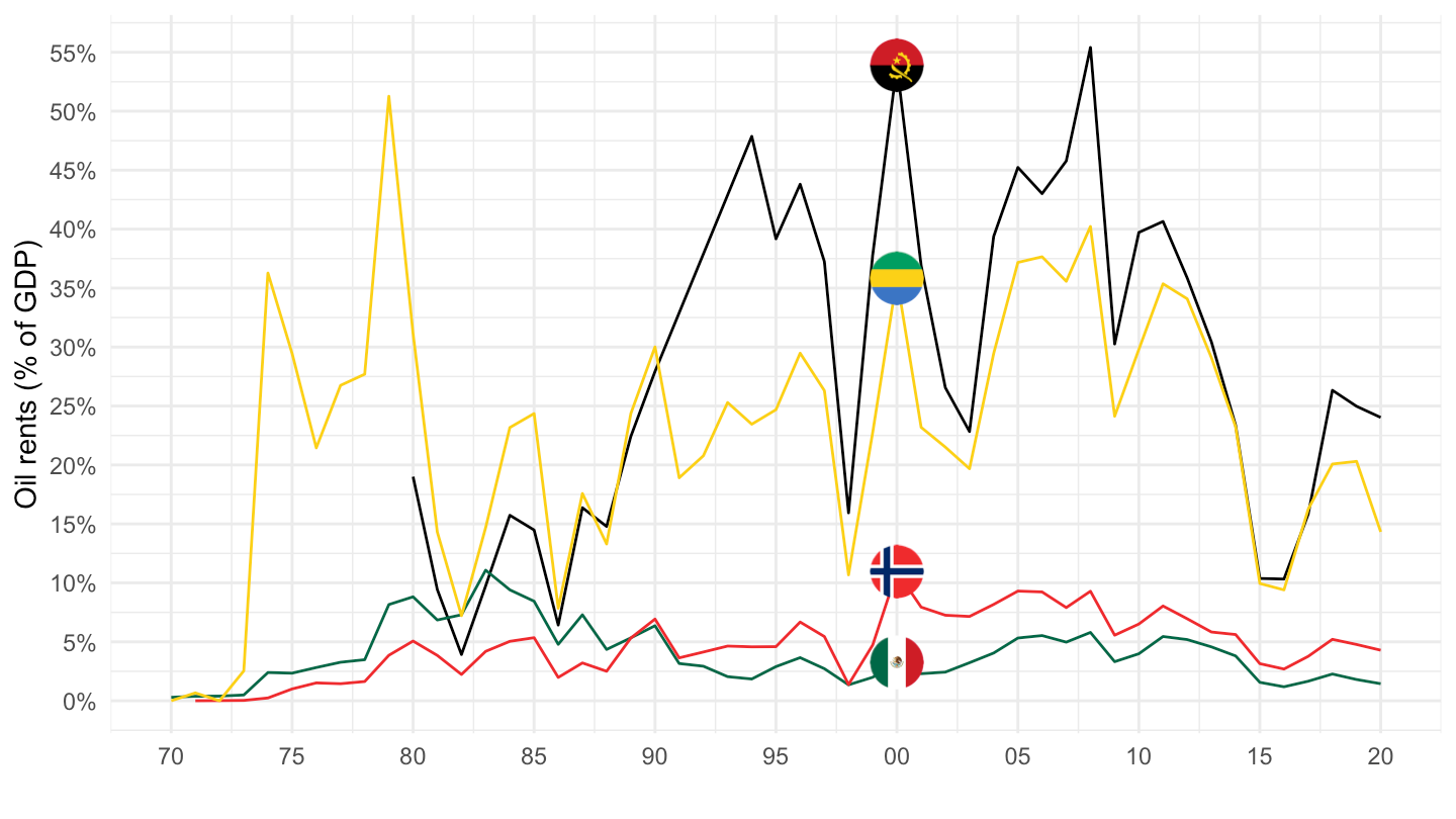
Kuwait, Iraq, Libya
NY.GDP.PETR.RT.ZS %>%
  filter(iso2c %in% c("KW", "IQ", "LY")) %>%
  left_join(iso2c, by = "iso2c") %>%
  year_to_date %>%
  mutate(value = NY.GDP.PETR.RT.ZS/100) %>%
  left_join(colors, by = c("Iso2c" = "country")) %>%
  ggplot(.) + geom_line(aes(x = date, y = value, color = color)) +
  scale_color_identity() + add_3flags + theme_minimal() +
  theme(legend.title = element_blank(),
        legend.position = c(0.5, 0.9),
        legend.direction = "horizontal") +
  scale_x_date(breaks = seq(1950, 2020, 5) %>% paste0("-01-01") %>% as.Date,
               labels = date_format("%y")) +
  scale_y_continuous(breaks = 0.01*seq(-60, 100, 5),
                     labels = scales::percent_format(accuracy = 1)) +
  xlab("") + ylab("Oil rents (% of GDP)")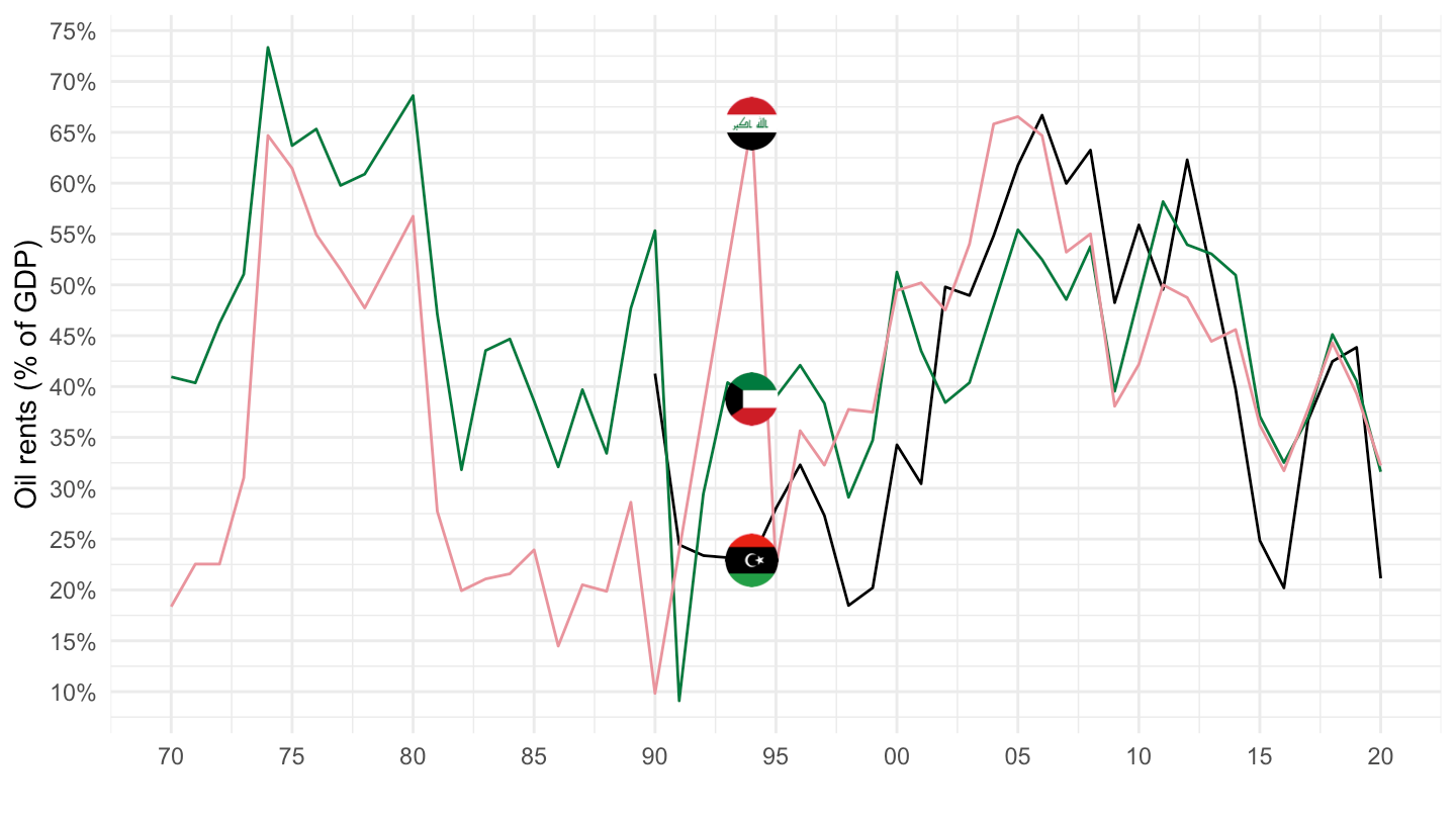
China, France, Germany
NY.GDP.PETR.RT.ZS %>%
  filter(iso2c %in% c("CN", "FR", "DE")) %>%
  left_join(iso2c, by = "iso2c") %>%
  year_to_date %>%
  mutate(value = NY.GDP.PETR.RT.ZS/100) %>%
  left_join(colors, by = c("Iso2c" = "country")) %>%
  ggplot(.) + geom_line(aes(x = date, y = value, color = color)) +
  scale_color_identity() + add_3flags + theme_minimal() +
  scale_x_date(breaks = seq(1950, 2020, 5) %>% paste0("-01-01") %>% as.Date,
               labels = date_format("%y")) +
  scale_y_continuous(breaks = 0.01*seq(-60, 60, 2),
                     labels = scales::percent_format(accuracy = 1)) +
  xlab("") + ylab("Oil rents (% of GDP)")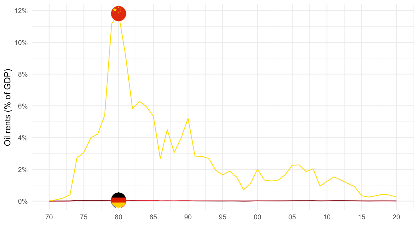
Spain, United Kingdom, United States
NY.GDP.PETR.RT.ZS %>%
  filter(iso2c %in% c("US", "GB", "ES")) %>%
  left_join(iso2c, by = "iso2c") %>%
  year_to_date %>%
  mutate(value = NY.GDP.PETR.RT.ZS/100) %>%
  left_join(colors, by = c("Iso2c" = "country")) %>%
  ggplot(.) + geom_line(aes(x = date, y = value, color = color)) +
  scale_color_identity() + add_3flags + theme_minimal() +
  scale_x_date(breaks = seq(1950, 2020, 5) %>% paste0("-01-01") %>% as.Date,
               labels = date_format("%y")) +
  scale_y_continuous(breaks = 0.01*seq(-60, 60, 1),
                     labels = scales::percent_format(accuracy = 1)) +
  xlab("") + ylab("Oil rents (% of GDP)")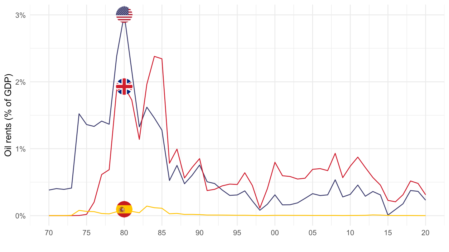
Argentina, Chile, Venezuela
NY.GDP.PETR.RT.ZS %>%
  filter(iso2c %in% c("AR", "CL", "VE")) %>%
  left_join(iso2c, by = "iso2c") %>%
  mutate(Iso2c = ifelse(iso2c == "VE", "Venezuela", Iso2c)) %>%
  year_to_date %>%
  mutate(value = NY.GDP.PETR.RT.ZS/100) %>%
  left_join(colors, by = c("Iso2c" = "country")) %>%
  ggplot(.) + geom_line(aes(x = date, y = value, color = color)) +
  scale_color_identity() + add_3flags + theme_minimal() +
  scale_x_date(breaks = seq(1950, 2020, 5) %>% paste0("-01-01") %>% as.Date,
               labels = date_format("%y")) +
  scale_y_continuous(breaks = 0.01*seq(-60, 60, 5),
                     labels = scales::percent_format(accuracy = 1)) +
  xlab("") + ylab("Oil rents (% of GDP)")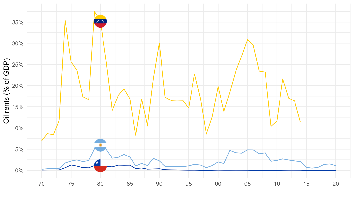
Greece, Hong Kong, Mexico
NY.GDP.PETR.RT.ZS %>%
  filter(iso2c %in% c("GR", "HK", "MX")) %>%
  left_join(iso2c, by = "iso2c") %>%
  mutate(Iso2c = ifelse(iso2c == "HK", "Hong Kong", Iso2c)) %>%
  year_to_date %>%
  mutate(value = NY.GDP.PETR.RT.ZS/100) %>%
  left_join(colors, by = c("Iso2c" = "country")) %>%
  ggplot(.) + geom_line(aes(x = date, y = value, color = color)) +
  scale_color_identity() + add_3flags + theme_minimal() +
  scale_x_date(breaks = seq(1950, 2020, 5) %>% paste0("-01-01") %>% as.Date,
               labels = date_format("%y")) +
  scale_y_continuous(breaks = 0.01*seq(-60, 60, 2),
                     labels = scales::percent_format(accuracy = 1)) +
  xlab("") + ylab("Oil rents (% of GDP)")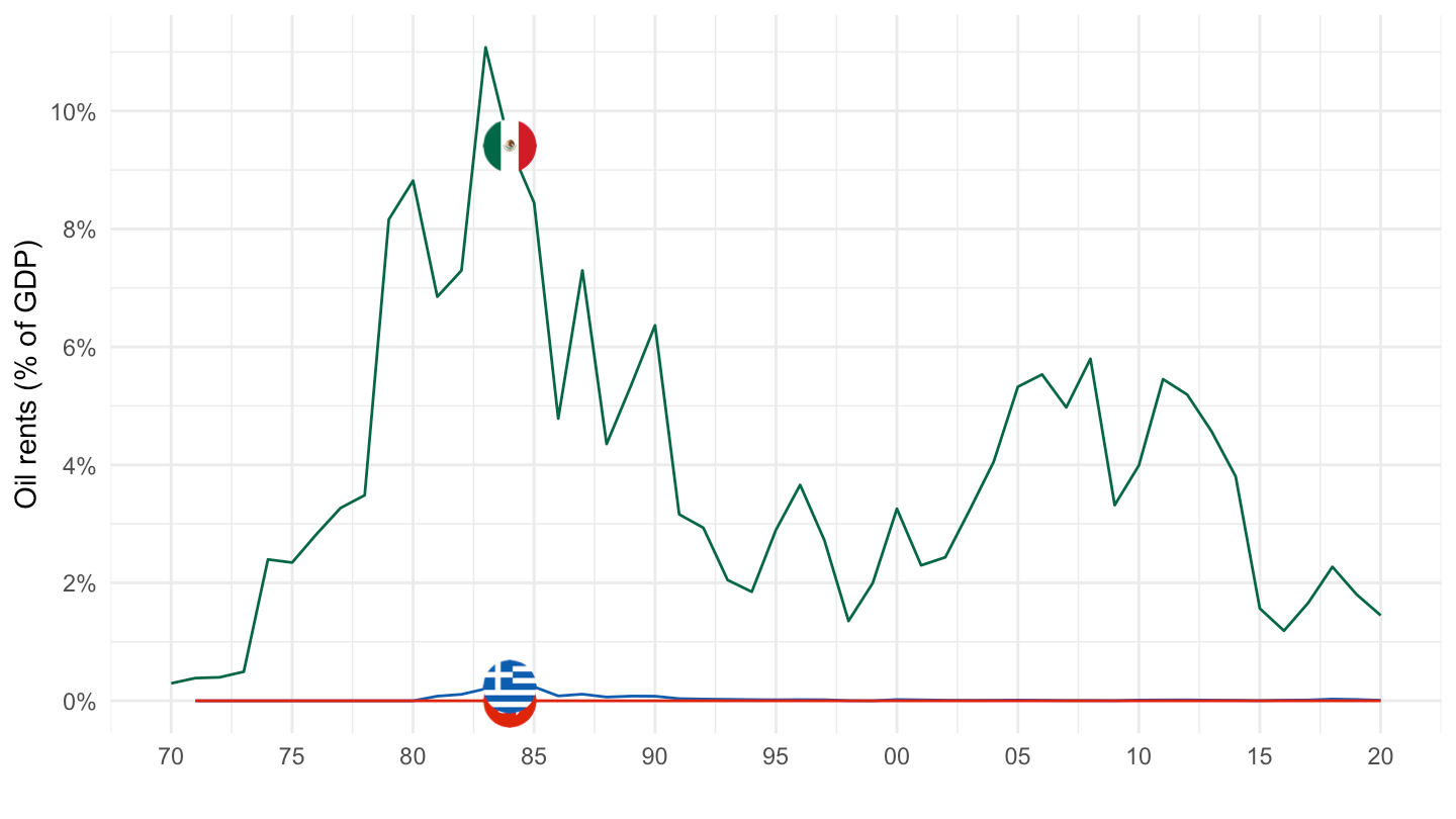
Map
Asia
library(WDI)
library(ggthemes)
library("rnaturalearth")
library(viridis)
library(WDI)
asia_map <- ne_countries(scale = "medium", continent = 'Asia', returnclass = "sf")
nat_rents = WDI(indicator='NY.GDP.TOTL.RT.ZS', start=2016, end=2018)
asia_rents <- merge(asia_map, nat_rents, by.x = "iso_a2", by.y = "iso2c", all = TRUE)
map_2017 <- asia_rents[which(asia_rents$year == 2017),]
nat_rent_graph <- ggplot(data = map_2017) +
  geom_sf(aes(fill = NY.GDP.TOTL.RT.ZS),
          position = "identity") +
  labs(fill ='Natural Resource Rents as % GDP') +
  scale_fill_viridis_c(option = "viridis")

nat_rent_graph + theme_map()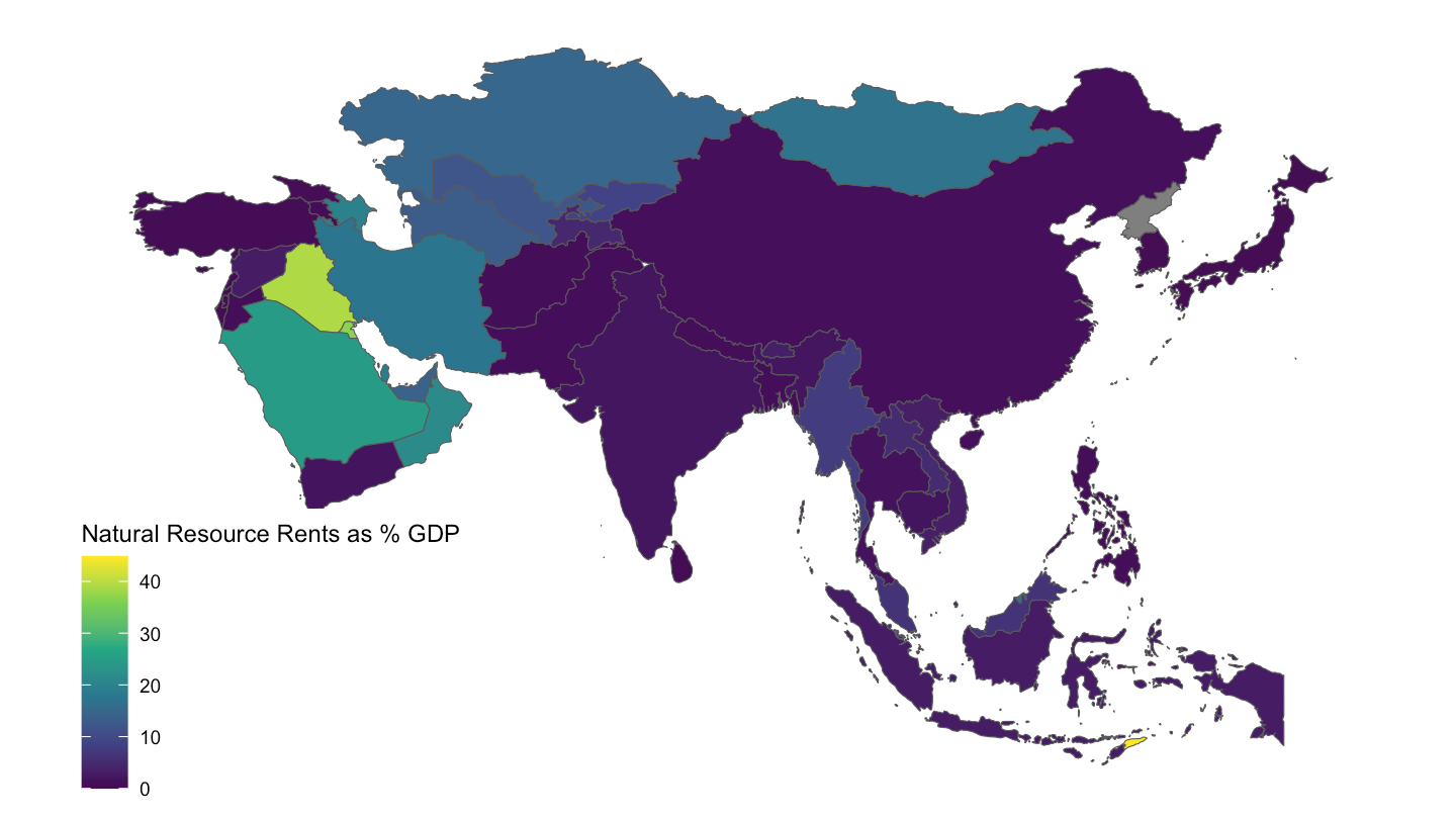
South America
library(WDI)
library(ggthemes)
library("rnaturalearth")
library(viridis)
library(WDI)
asia_map <- ne_countries(scale = "medium", continent = 'South America', returnclass = "sf")
nat_rents = WDI(indicator='NY.GDP.TOTL.RT.ZS', start=2016, end=2018)
asia_rents <- merge(asia_map, nat_rents, by.x = "iso_a2", by.y = "iso2c", all = TRUE)
map_2017 <- asia_rents[which(asia_rents$year == 2017),]
nat_rent_graph <- ggplot(data = map_2017) +
  geom_sf(aes(fill = NY.GDP.TOTL.RT.ZS),
          position = "identity") +
  labs(fill ='Natural Resource Rents as % GDP') +
  scale_fill_viridis_c(option = "viridis")

nat_rent_graph + theme_map()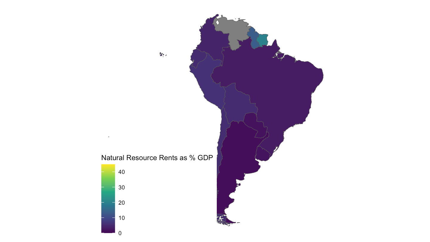
North America
library(WDI)
library(ggthemes)
library("rnaturalearth")
library(viridis)
library(WDI)
asia_map <- ne_countries(scale = "medium", continent = 'North America', returnclass = "sf")
nat_rents = WDI(indicator='NY.GDP.TOTL.RT.ZS', start=2016, end=2018)
asia_rents <- merge(asia_map, nat_rents, by.x = "iso_a2", by.y = "iso2c", all = TRUE)
map_2017 <- asia_rents[which(asia_rents$year == 2017),]
nat_rent_graph <- ggplot(data = map_2017) +
  geom_sf(aes(fill = NY.GDP.TOTL.RT.ZS),
          position = "identity") +
  labs(fill ='Natural Resource Rents as % GDP') +
  scale_fill_viridis_c(option = "viridis")

nat_rent_graph + theme_map()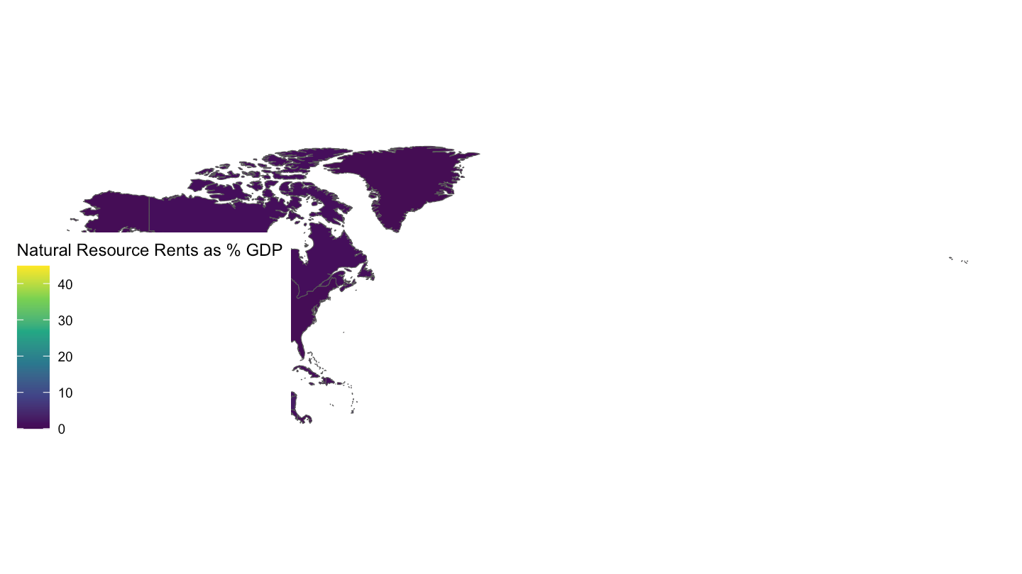
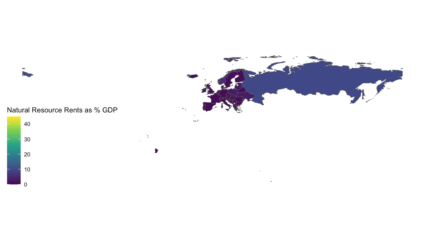
Europe
library(WDI)
library(ggthemes)
library("rnaturalearth")
library(viridis)
library(WDI)
asia_map <- ne_countries(scale = "medium", continent = 'Europe', returnclass = "sf")
nat_rents = WDI(indicator='NY.GDP.TOTL.RT.ZS', start=2016, end=2018)
asia_rents <- merge(asia_map, nat_rents, by.x = "iso_a2", by.y = "iso2c", all = TRUE)
map_2017 <- asia_rents[which(asia_rents$year == 2017),]
nat_rent_graph <- ggplot(data = map_2017) +
  geom_sf(aes(fill = NY.GDP.TOTL.RT.ZS),
          position = "identity") +
  labs(fill ='Natural Resource Rents as % GDP') +
  scale_fill_viridis_c(option = "viridis")

nat_rent_graph + theme_map()