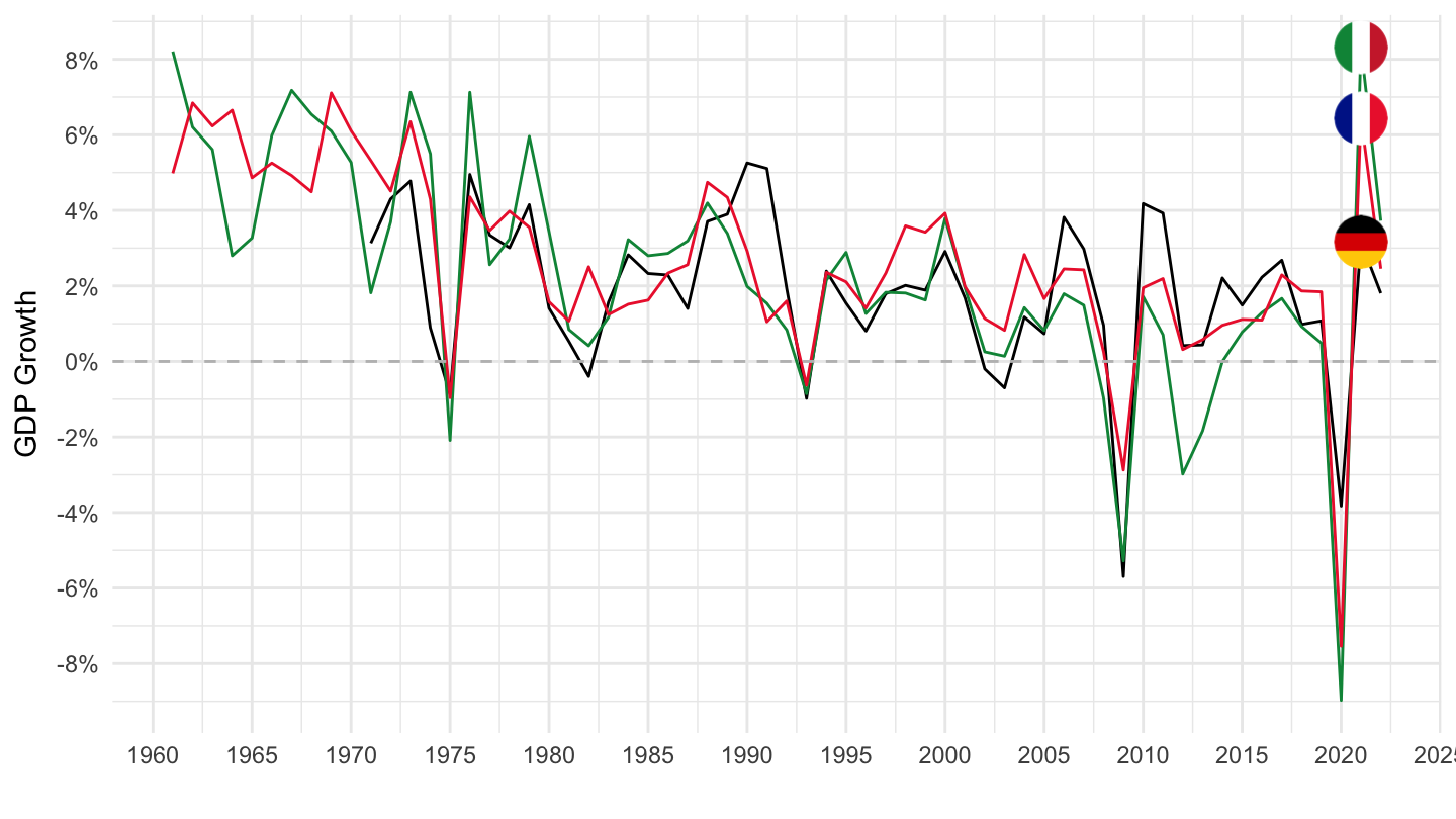
NY.GDP.MKTP.KD.ZG %>%
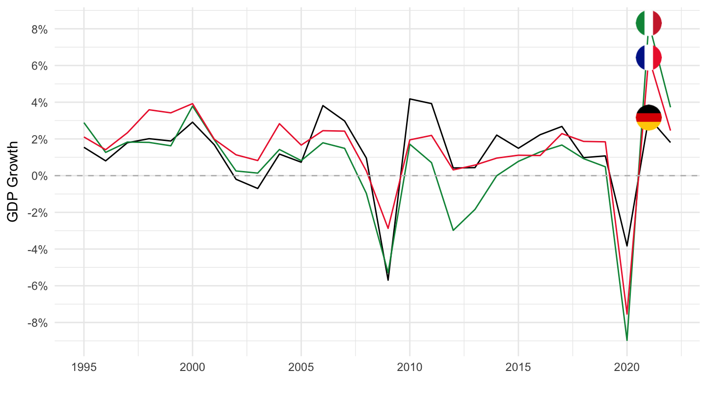
filter(iso2c %in% c("FR", "DE", "IT")) %>%
left_join(iso2c, by = "iso2c") %>%
year_to_date() %>%
mutate(value = value/100) %>%
left_join(colors, by = c("Iso2c" = "country")) %>%
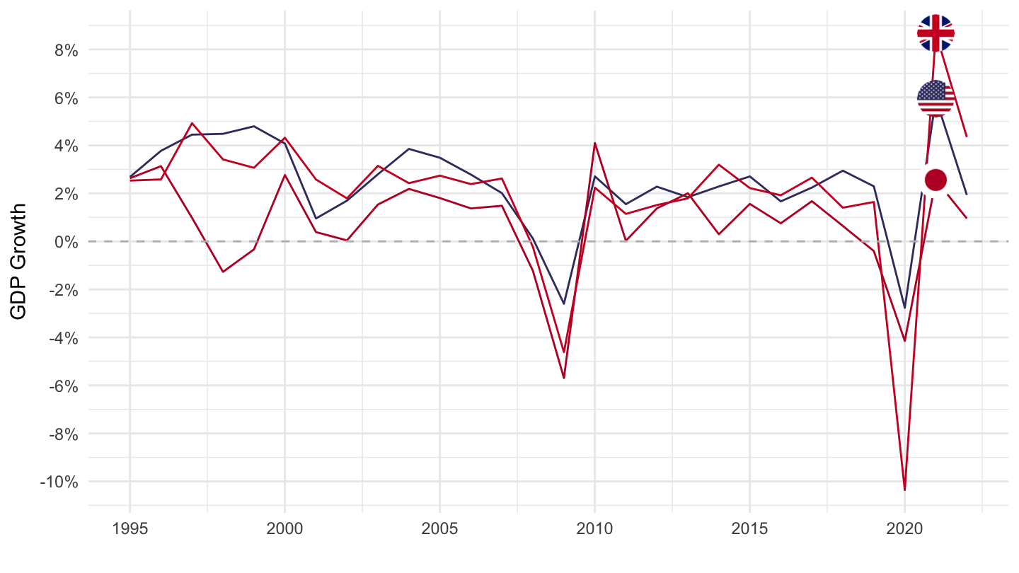
ggplot(.) + geom_line(aes(x = date, y = value, color = color)) +
theme_minimal() + xlab("") + ylab("GDP Growth") +
scale_color_identity() + add_flags +
theme(legend.title = element_blank(),
legend.position = c(0.6, 0.9),
legend.direction = "horizontal") +
scale_x_date(breaks = seq(1900, 2100, 5) %>% paste0("-01-01") %>% as.Date,
labels = date_format("%Y")) +
scale_y_continuous(breaks = 0.01*seq(-100, 10000, 2),
labels = percent_format(a = 1)) +
geom_hline(yintercept = 0, linetype = "dashed", color = "grey")