Last observation: 2024 (N = 192)
First observation: 1960 (N = 81)
Last data update: 04 oct. 2026, 23:33
Last compile: 04 oct. 2026, 23:48
MS.MIL.XPND.GD.ZS |>
  left_join(iso2c, by = "iso2c") |>
  group_by(iso2c, Iso2c) |>
  mutate(value = round(value, 1)) |>
  summarise(Nobs = n(),
            `Year 1` = first(year),
            `Manufacturing Share 1 (%)` = first(value),
            `Year 2` = last(year),
            `Manufacturing Share 2 (%)` = last(value)) |>
  arrange(-`Manufacturing Share 2 (%)`) |>
  mutate(Flag = gsub(" ", "-", str_to_lower(Iso2c)),
         Flag = paste0('<img src="../../bib/flags/vsmall/', Flag, '.png" alt="Flag">')) |>
  select(Flag, everything()) %>%
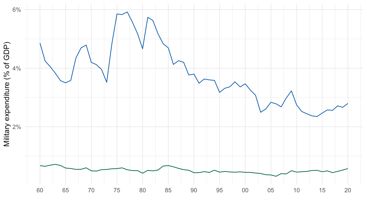
{if (is_html_output()) datatable(., filter = 'top', rownames = F, escape = F) else .}MS.MIL.XPND.GD.ZS |>
left_join(iso2c, by = "iso2c") |>
group_by(iso2c, Iso2c) |>
summarise(Period = paste0(first(year), "-", last(year)),
Nobs = n()) |>
arrange(-Nobs) %>%
{if (is_html_output()) datatable(., filter = 'top', rownames = F) else .}MS.MIL.XPND.GD.ZS |>
filter(iso2c %in% c("AF")) |>
left_join(iso2c, by = "iso2c") |>
year_to_date() |>
ggplot() + xlab("") + ylab("Military expenditure (% of GDP)") +
geom_line(aes(x = date, y = value/100)) + theme_minimal() +
theme(legend.title = element_blank(),
legend.position = c(0.2, 0.2)) +
scale_x_date(breaks = seq(1950, 2100, 2) |> paste0("-01-01") |> as.Date(),
labels = date_format("%Y")) +
scale_y_continuous(breaks = 0.01*seq(-60, 60, 2),
labels = scales::percent_format(accuracy = 1))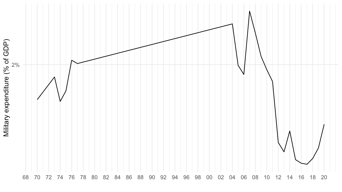
MS.MIL.XPND.GD.ZS |>
  filter(iso2c %in% c("AR")) |>
  left_join(iso2c, by = "iso2c") |>
  year_to_date() |>
  ggplot() + xlab("") + ylab("Military expenditure (% of GDP)") +
  geom_line(aes(x = date, y = value/100)) + theme_minimal() +
  theme(legend.title = element_blank(),
        legend.position = c(0.2, 0.2)) +
  scale_x_date(breaks = seq(1950, 2100, 2) |> paste0("-01-01") |> as.Date(),
               labels = date_format("%Y")) +
  scale_y_continuous(breaks = 0.01*seq(-60, 60, 2),
                     labels = scales::percent_format(accuracy = 1))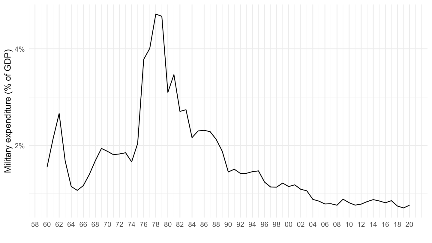
MS.MIL.XPND.GD.ZS |>
  filter(iso2c %in% c("UY")) |>
  left_join(iso2c, by = "iso2c") |>
  year_to_date() |>
  ggplot() + xlab("") + ylab("Military expenditure (% of GDP)") +
  geom_line(aes(x = date, y = value/100)) + theme_minimal() +
  theme(legend.title = element_blank(),
        legend.position = c(0.2, 0.2)) +
  scale_x_date(breaks = seq(1950, 2100, 2) |> paste0("-01-01") |> as.Date(),
               labels = date_format("%Y")) +
  scale_y_continuous(breaks = 0.01*seq(-60, 60, 2),
                     labels = scales::percent_format(accuracy = 1))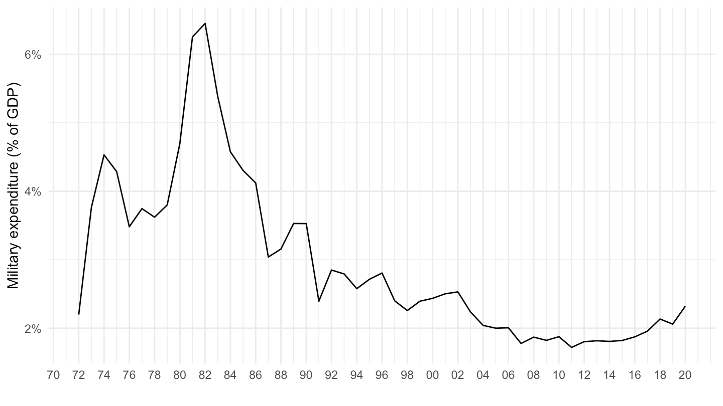
MS.MIL.XPND.GD.ZS |>
  filter(iso2c %in% c("HU")) |>
  left_join(iso2c, by = "iso2c") |>
  year_to_date() |>
  ggplot() + xlab("") + ylab("Military expenditure (% of GDP)") +
  geom_line(aes(x = date, y = value/100)) + theme_minimal() +
  theme(legend.title = element_blank(),
        legend.position = c(0.2, 0.2)) +
  scale_x_date(breaks = seq(1950, 2100, 2) |> paste0("-01-01") |> as.Date(),
               labels = date_format("%Y")) +
  scale_y_continuous(breaks = 0.01*seq(-60, 60, 0.5),
                     labels = scales::percent_format(accuracy = 0.1))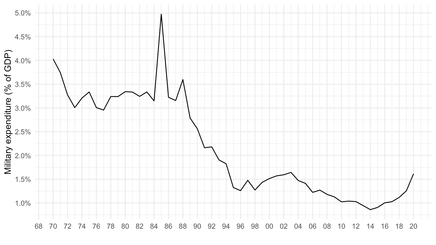
MS.MIL.XPND.GD.ZS |>
  filter(iso2c %in% c("OE", "1W", "EU")) |>
  left_join(iso2c, by = "iso2c") |>
  year_to_date() |>
  mutate(Iso2c = ifelse(iso2c == "OE", "OECD Members", Iso2c)) |>
  add_flag_color("Iso2c") |>
  mutate(value = value/100) |>
  ggplot() + geom_line(aes(x = date, y = value, color = color)) +
  xlab("") + ylab("Military expenditure (% of GDP)") +
  theme_minimal() + scale_color_identity() + add_flags +
  scale_x_date(breaks = seq(1950, 2100, 5) |> paste0("-01-01") |> as.Date(),
               labels = date_format("%Y")) +
  scale_y_continuous(breaks = 0.01*seq(-60, 60, 1),
                     labels = scales::percent_format(accuracy = 1))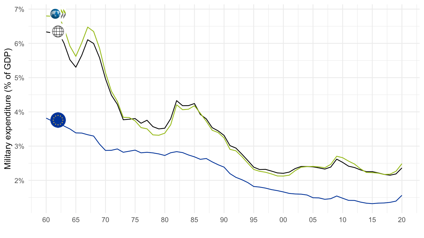
MS.MIL.XPND.GD.ZS |>
  filter(iso2c %in% c("OE", "1W", "EU", "SE")) |>
  left_join(iso2c, by = "iso2c") |>
  year_to_date() |>
  mutate(Iso2c = ifelse(iso2c == "OE", "OECD Members", Iso2c)) |>
  add_flag_color("Iso2c") |>
  mutate(value = value/100) |>
  ggplot() + geom_line(aes(x = date, y = value, color = color)) +
  xlab("") + ylab("Military expenditure (% of GDP)") +
  theme_minimal() + scale_color_identity() + add_flags +
  scale_x_date(breaks = seq(1950, 2100, 5) |> paste0("-01-01") |> as.Date(),
               labels = date_format("%Y")) +
  scale_y_continuous(breaks = 0.01*seq(-60, 60, 1),
                     labels = scales::percent_format(accuracy = 1))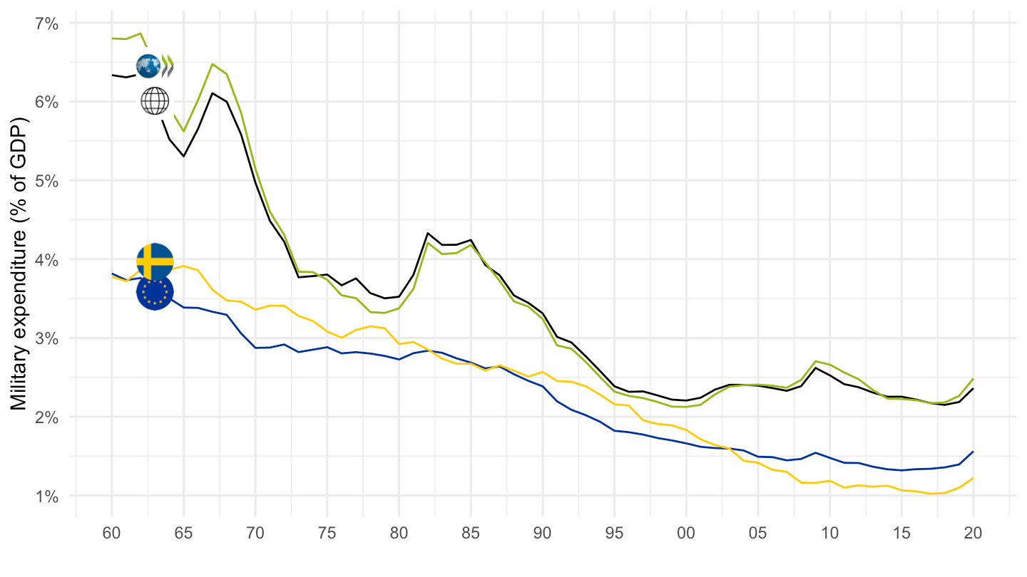
MS.MIL.XPND.GD.ZS |>
  filter(iso2c %in% c("OE", "FR", "DE", "US", "GB")) |>
  left_join(iso2c, by = "iso2c") |>
  year_to_date() |>
  mutate(Iso2c = ifelse(iso2c == "OE", "OECD Members", Iso2c)) |>
  add_flag_color("Iso2c") |>
  mutate(value = value/100) |>
  ggplot() + geom_line(aes(x = date, y = value, color = color)) +
  xlab("") + ylab("Military expenditure (% of GDP)") +
  theme_minimal() + scale_color_identity() + add_flags +
  scale_x_date(breaks = seq(1950, 2100, 5) |> paste0("-01-01") |> as.Date(),
               labels = date_format("%Y")) +
  scale_y_continuous(breaks = 0.01*seq(-60, 60, 1),
                     labels = scales::percent_format(accuracy = 1))
MS.MIL.XPND.GD.ZS |>
  filter(iso2c %in% c("OE", "FR", "DE", "US", "GB")) |>
  left_join(iso2c, by = "iso2c") |>
  year_to_date() |>
  filter(date >= as.Date("1995-01-01")) |>
  mutate(Iso2c = ifelse(iso2c == "OE", "OECD Members", Iso2c)) |>
  add_flag_color("Iso2c") |>
  mutate(value = value/100) |>
  ggplot() + geom_line(aes(x = date, y = value, color = color)) +
  xlab("") + ylab("Military expenditure (% of GDP)") +
  theme_minimal() + scale_color_identity() + add_flags +
  scale_x_date(breaks = seq(1950, 2100, 2) |> paste0("-01-01") |> as.Date(),
               labels = date_format("%Y")) +
  scale_y_continuous(breaks = 0.01*seq(-60, 60, 1),
                     labels = scales::percent_format(accuracy = 1))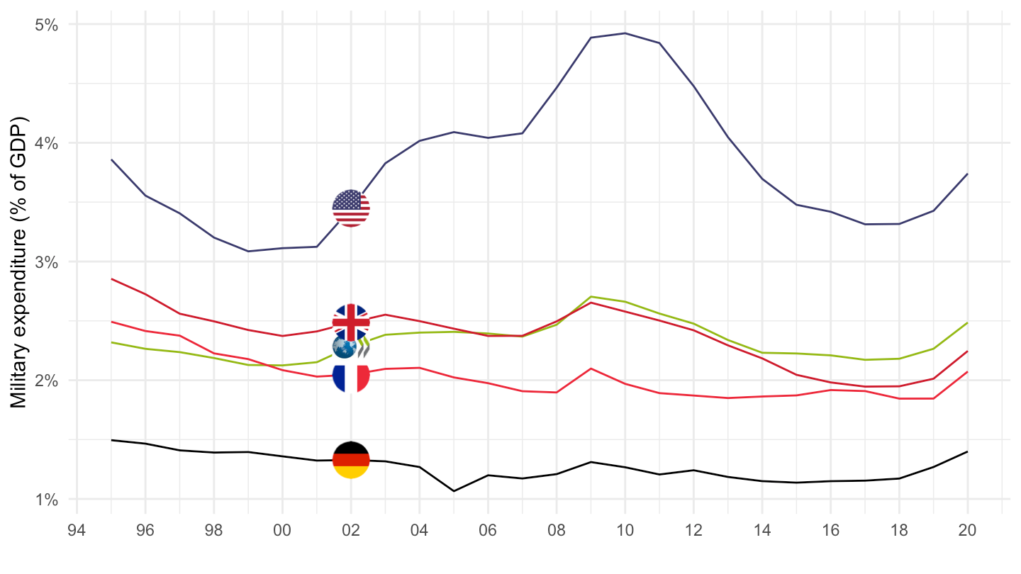
MS.MIL.XPND.GD.ZS |>
  filter(iso2c %in% c("OE", "1W", "FR", "DE", "US", "GB", "RU")) |>
  left_join(iso2c, by = "iso2c") |>
  year_to_date() |>
  mutate(Iso2c = ifelse(iso2c == "OE", "OECD Members", Iso2c)) |>
  mutate(Iso2c = ifelse(iso2c == "RU", "Russia", Iso2c)) |>
  add_flag_color("Iso2c") |>
  mutate(value = value/100) |>
  ggplot() + geom_line(aes(x = date, y = value, color = color)) +
  xlab("") + ylab("Military expenditure (% of GDP)") +
  theme_minimal() + scale_color_identity() + add_flags +
  scale_x_date(breaks = seq(1950, 2100, 5) |> paste0("-01-01") |> as.Date(),
               labels = date_format("%Y")) +
  scale_y_continuous(breaks = 0.01*seq(-60, 60, 1),
                     labels = scales::percent_format(accuracy = 1))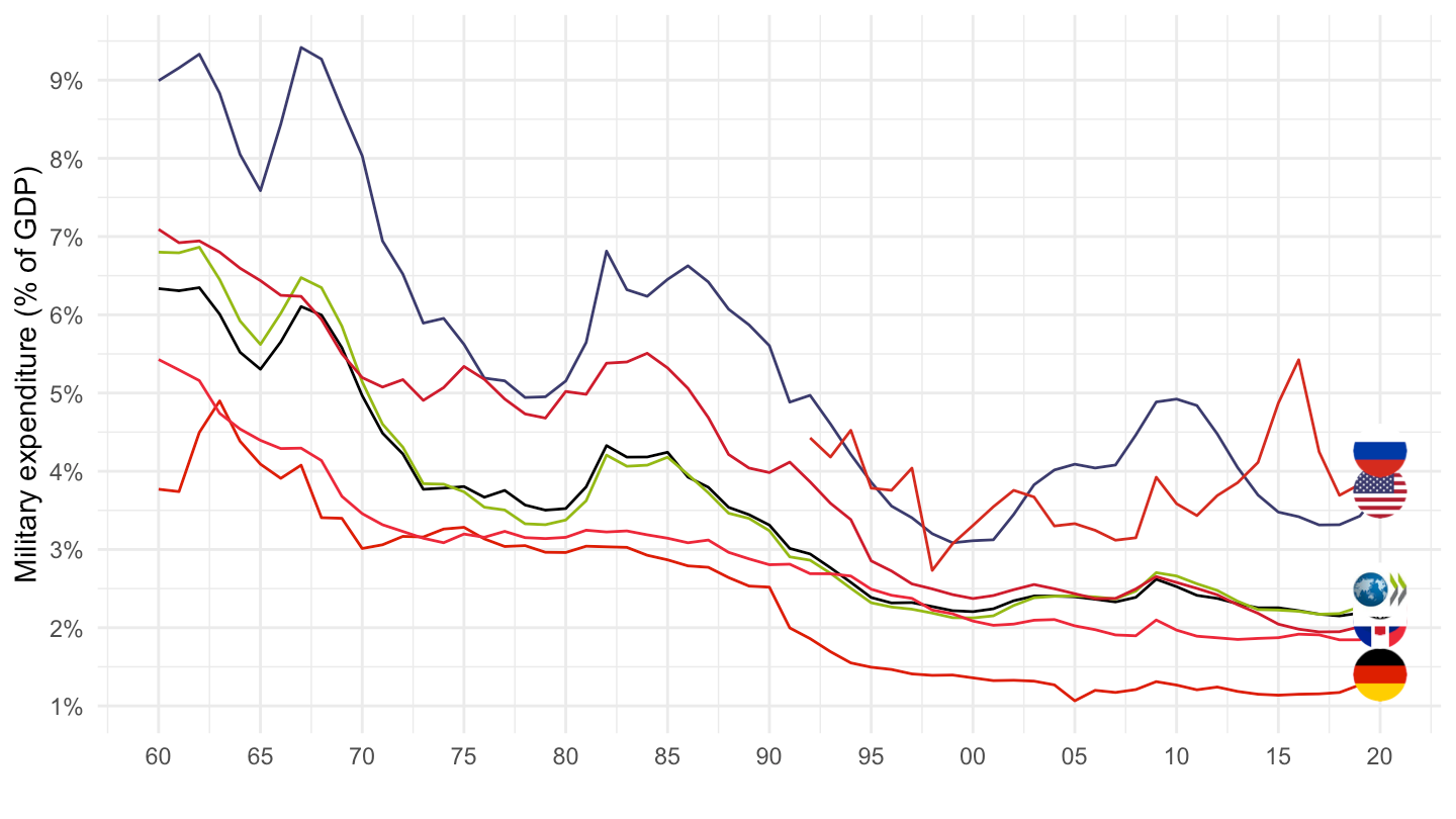
MS.MIL.XPND.GD.ZS |>
  filter(iso2c %in% c("OE", "1W", "FR", "DE", "US", "GB", "RU")) |>
  left_join(iso2c, by = "iso2c") |>
  year_to_date() |>
  filter(date >= as.Date("1995-01-01")) |>
  mutate(Iso2c = ifelse(iso2c == "OE", "OECD Members", Iso2c)) |>
  mutate(Iso2c = ifelse(iso2c == "RU", "Russia", Iso2c)) |>
  add_flag_color("Iso2c") |>
  mutate(value = value/100) |>
  ggplot() + geom_line(aes(x = date, y = value, color = color)) +
  xlab("") + ylab("Military expenditure (% of GDP)") +
  theme_minimal() + scale_color_identity() + add_flags +
  scale_x_date(breaks = seq(1950, 2100, 2) |> paste0("-01-01") |> as.Date(),
               labels = date_format("%Y")) +
  scale_y_continuous(breaks = 0.01*seq(-60, 60, 1),
                     labels = scales::percent_format(accuracy = 1))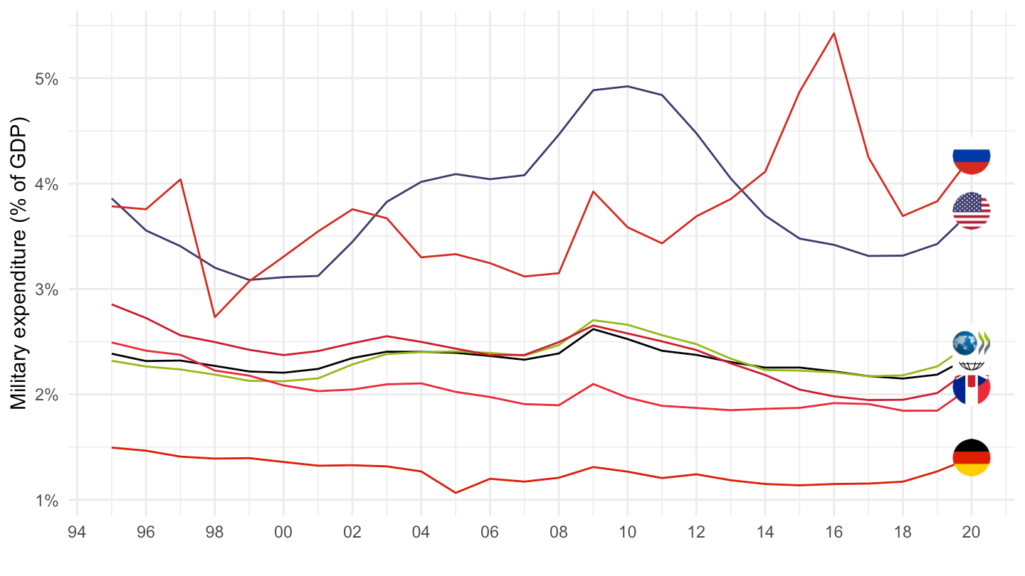
MS.MIL.XPND.GD.ZS |>
  filter(iso2c %in% c("OE", "1W", "FR", "DE", "US", "GB")) |>
  left_join(iso2c, by = "iso2c") |>
  year_to_date() |>
  mutate(Iso2c = ifelse(iso2c == "OE", "OECD Members", Iso2c)) |>
  add_flag_color("Iso2c") |>
  mutate(value = value/100) |>
  ggplot() + geom_line(aes(x = date, y = value, color = color)) +
  xlab("") + ylab("Military expenditure (% of GDP)") +
  theme_minimal() + scale_color_identity() + add_flags +
  scale_x_date(breaks = seq(1950, 2100, 5) |> paste0("-01-01") |> as.Date(),
               labels = date_format("%Y")) +
  scale_y_continuous(breaks = 0.01*seq(-60, 60, 1),
                     labels = scales::percent_format(accuracy = 1))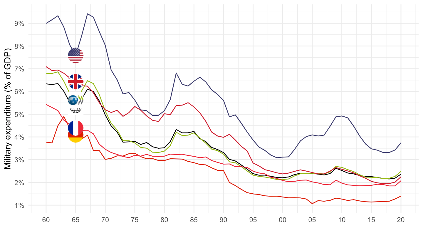
MS.MIL.XPND.GD.ZS |>
  filter(iso2c %in% c("OE", "1W", "FR", "DE", "US", "GB")) |>
  left_join(iso2c, by = "iso2c") |>
  year_to_date() |>
  filter(date >= as.Date("1995-01-01")) |>
  mutate(Iso2c = ifelse(iso2c == "OE", "OECD Members", Iso2c)) |>
  add_flag_color("Iso2c") |>
  mutate(value = value/100) |>
  ggplot() + geom_line(aes(x = date, y = value, color = color)) +
  xlab("") + ylab("Military expenditure (% of GDP)") +
  theme_minimal() + scale_color_identity() + add_flags +
  scale_x_date(breaks = seq(1950, 2100, 2) |> paste0("-01-01") |> as.Date(),
               labels = date_format("%Y")) +
  scale_y_continuous(breaks = 0.01*seq(-60, 60, 1),
                     labels = scales::percent_format(accuracy = 1))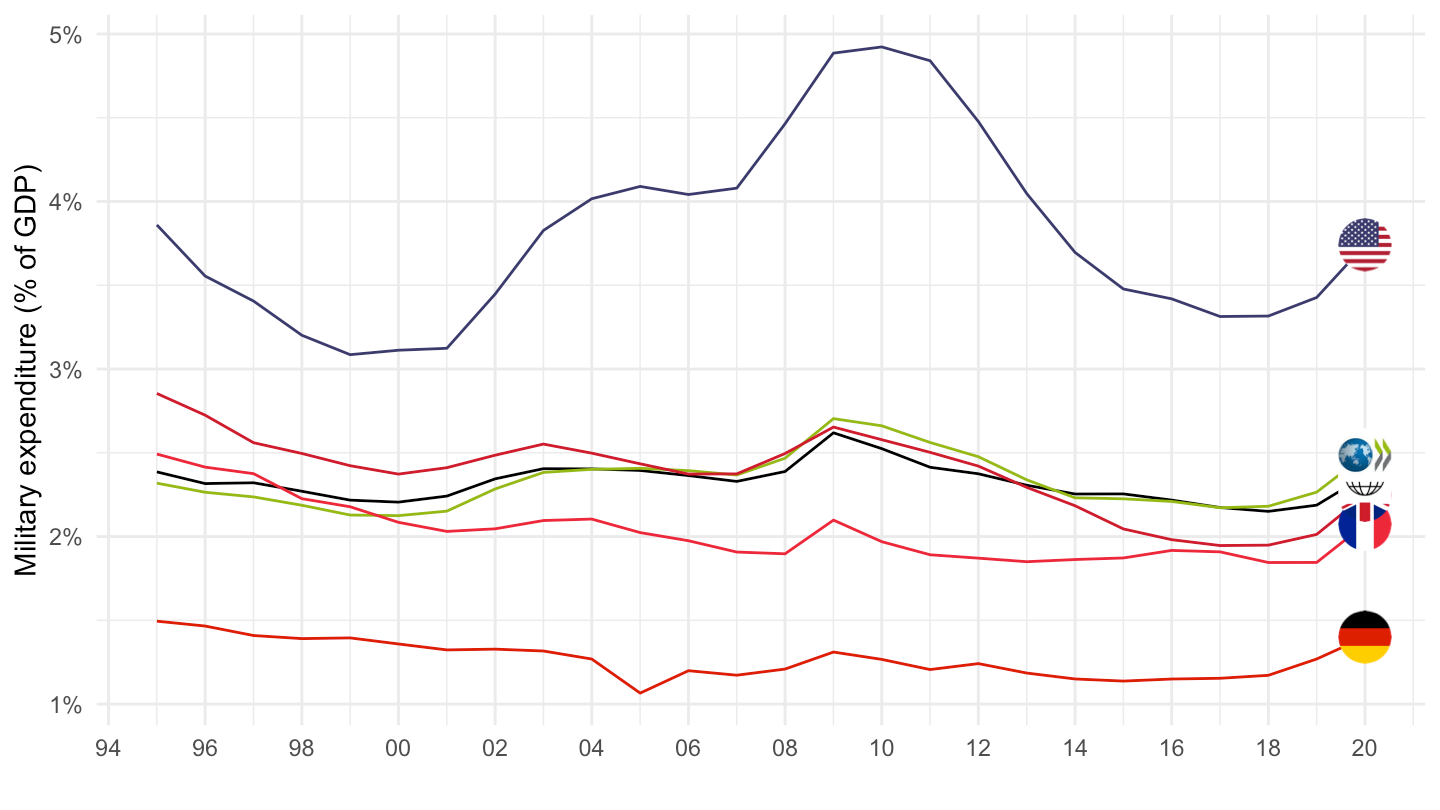
MS.MIL.XPND.GD.ZS |>
  filter(iso2c %in% c("OE", "1W", "FR", "DE", "US", "GB", "CN")) |>
  left_join(iso2c, by = "iso2c") |>
  year_to_date() |>
  filter(date >= as.Date("1995-01-01")) |>
  mutate(Iso2c = ifelse(iso2c == "OE", "OECD Members", Iso2c)) |>
  add_flag_color("Iso2c") |>
  mutate(value = value/100) |>
  ggplot() + geom_line(aes(x = date, y = value, color = color)) +
  xlab("") + ylab("Military expenditure (% of GDP)") +
  theme_minimal() + scale_color_identity() + add_flags +
  scale_x_date(breaks = seq(1950, 2100, 2) |> paste0("-01-01") |> as.Date(),
               labels = date_format("%Y")) +
  scale_y_continuous(breaks = 0.01*seq(-60, 60, 1),
                     labels = scales::percent_format(accuracy = 1))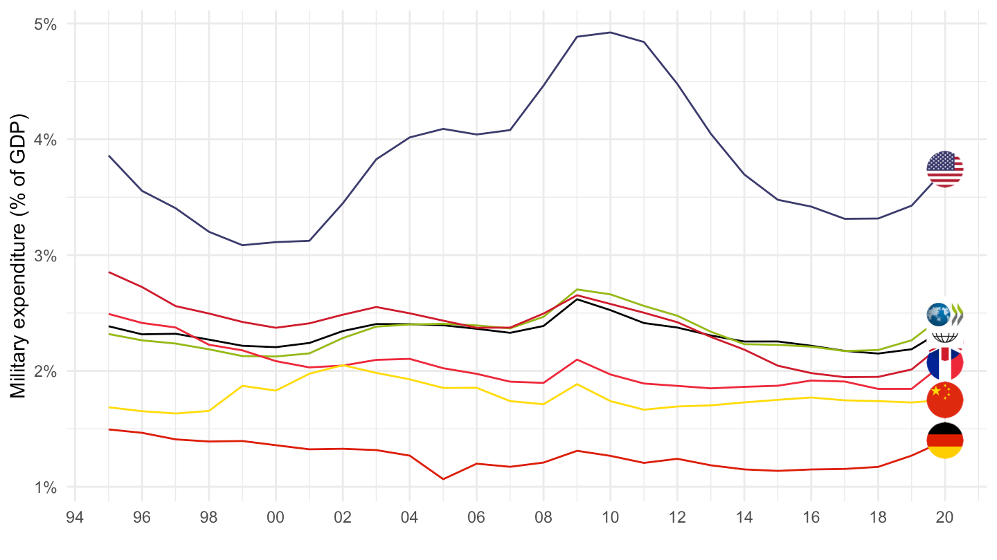
MS.MIL.XPND.GD.ZS |>
  filter(iso2c %in% c("OE", "1W", "FR", "DE")) |>
  left_join(iso2c, by = "iso2c") |>
  year_to_date() |>
  mutate(Iso2c = ifelse(iso2c == "OE", "OECD Members", Iso2c)) |>
  add_flag_color("Iso2c") |>
  mutate(value = value/100) |>
  ggplot() + geom_line(aes(x = date, y = value, color = color)) +
  xlab("") + ylab("Military expenditure (% of GDP)") +
  theme_minimal() + scale_color_identity() + add_flags +
  scale_x_date(breaks = seq(1950, 2100, 5) |> paste0("-01-01") |> as.Date(),
               labels = date_format("%Y")) +
  scale_y_continuous(breaks = 0.01*seq(-60, 60, 1),
                     labels = scales::percent_format(accuracy = 1))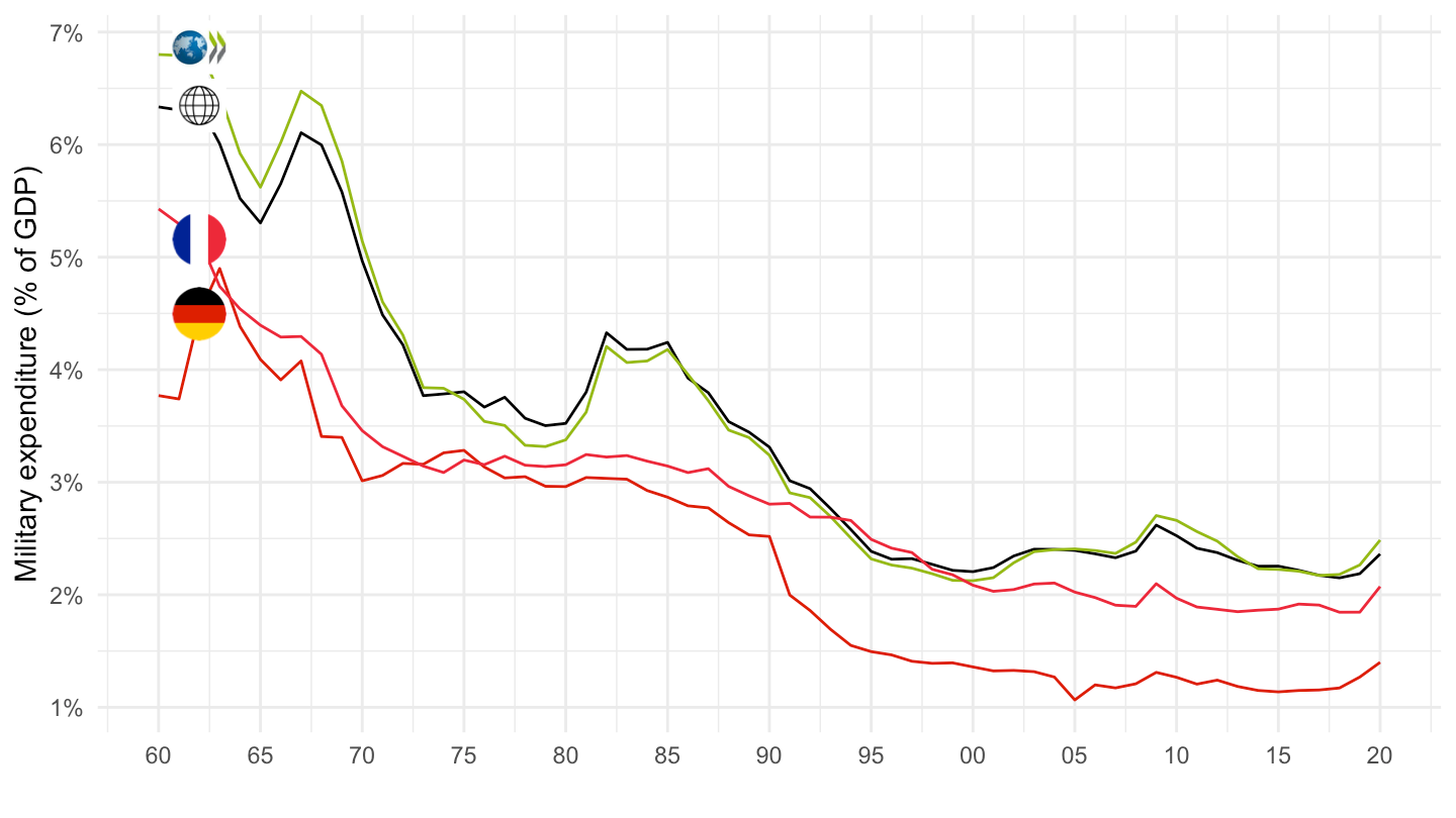
MS.MIL.XPND.GD.ZS |>
  filter(iso2c %in% c("OE", "1W", "FR", "DE")) |>
  left_join(iso2c, by = "iso2c") |>
  year_to_date() |>
  filter(date >= as.Date("1997-01-01")) |>
  mutate(Iso2c = ifelse(iso2c == "OE", "OECD Members", Iso2c)) |>
  add_flag_color("Iso2c") |>
  mutate(value = value/100) |>
  ggplot() + geom_line(aes(x = date, y = value, color = color)) +
  xlab("") + ylab("Military expenditure (% of GDP)") +
  theme_minimal() + scale_color_identity() + add_flags +
  scale_x_date(breaks = seq(1950, 2100, 5) |> paste0("-01-01") |> as.Date(),
               labels = date_format("%Y")) +
  scale_y_continuous(breaks = 0.01*seq(-60, 60, 1),
                     labels = scales::percent_format(accuracy = 1))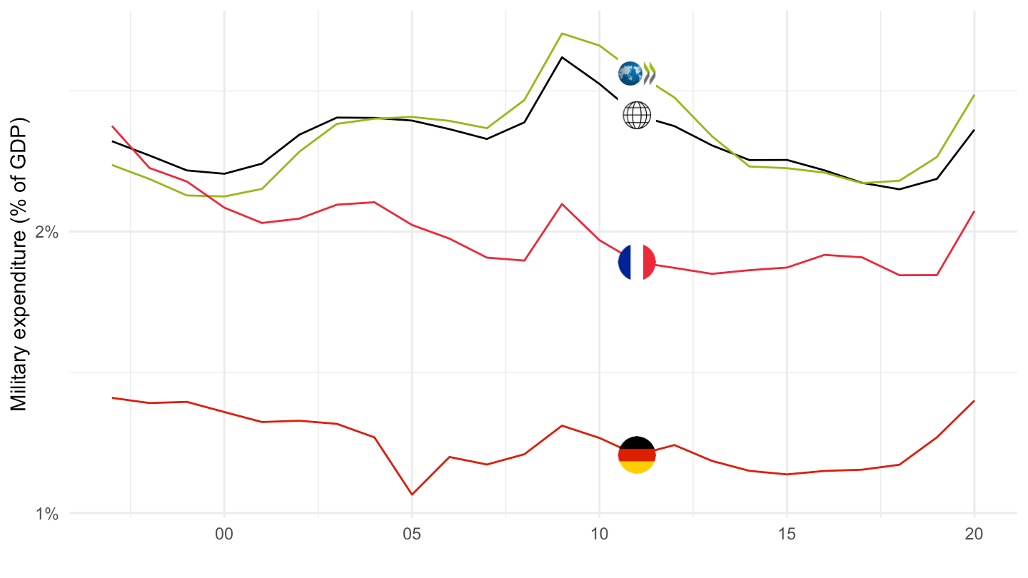
MS.MIL.XPND.GD.ZS |>
  filter(iso2c %in% c("OE", "FR", "DE")) |>
  left_join(iso2c, by = "iso2c") |>
  year_to_date() |>
  mutate(Iso2c = ifelse(iso2c == "OE", "OECD Members", Iso2c)) |>
  add_flag_color("Iso2c") |>
  mutate(value = value/100) |>
  ggplot() + geom_line(aes(x = date, y = value, color = color)) +
  xlab("") + ylab("Military expenditure (% of GDP)") +
  theme_minimal() + scale_color_identity() + add_flags +
  scale_x_date(breaks = seq(1950, 2100, 5) |> paste0("-01-01") |> as.Date(),
               labels = date_format("%Y")) +
  scale_y_continuous(breaks = 0.01*seq(-60, 60, 2),
                     labels = scales::percent_format(accuracy = 1))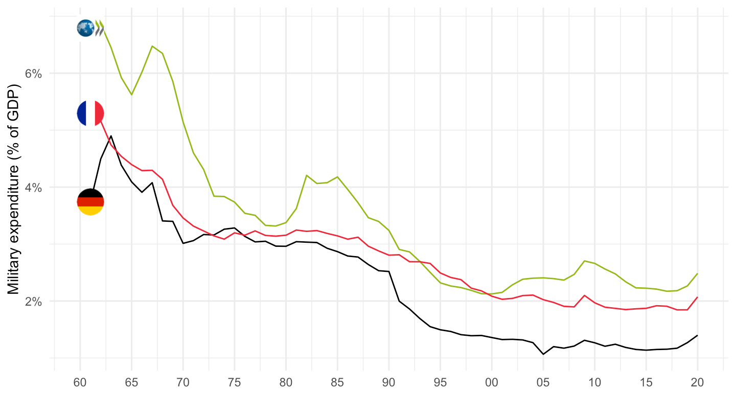
MS.MIL.XPND.GD.ZS |>
  filter(iso2c %in% c("CN", "FR", "DE")) |>
  left_join(iso2c, by = "iso2c") |>
  year_to_date() |>
  add_flag_color("Iso2c") |>
  mutate(value = value/100) |>
  ggplot() + geom_line(aes(x = date, y = value, color = color)) +
  xlab("") + ylab("Military expenditure (% of GDP)") +
  theme_minimal() + scale_color_identity() + add_flags +
  scale_x_date(breaks = seq(1950, 2100, 5) |> paste0("-01-01") |> as.Date(),
               labels = date_format("%Y")) +
  scale_y_continuous(breaks = 0.01*seq(-60, 60, 2),
                     labels = scales::percent_format(accuracy = 1))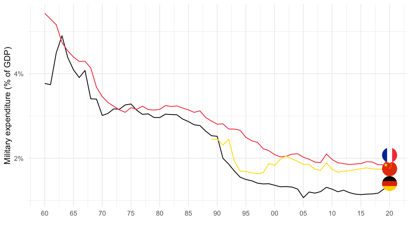
MS.MIL.XPND.GD.ZS |>
  filter(iso2c %in% c("SE", "FR", "DE")) |>
  left_join(iso2c, by = "iso2c") |>
  year_to_date() |>
  add_flag_color("Iso2c") |>
  mutate(value = value/100) |>
  ggplot() + geom_line(aes(x = date, y = value, color = color)) +
  xlab("") + ylab("Military expenditure (% of GDP)") +
  theme_minimal() + scale_color_identity() + add_flags +
  scale_x_date(breaks = seq(1950, 2100, 5) |> paste0("-01-01") |> as.Date(),
               labels = date_format("%Y")) +
  scale_y_continuous(breaks = 0.01*seq(-60, 60, 2),
                     labels = scales::percent_format(accuracy = 1))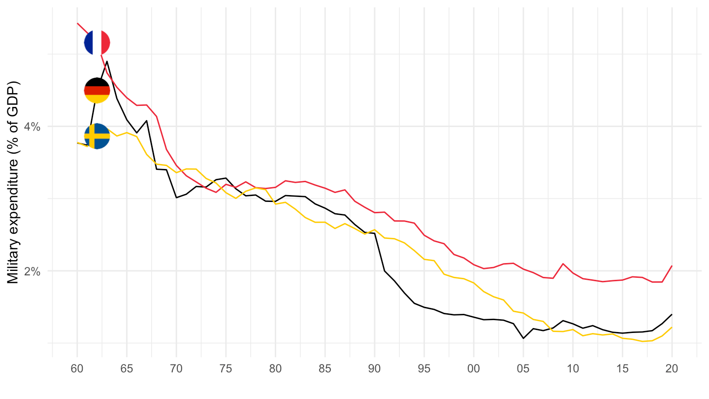
MS.MIL.XPND.GD.ZS |>
  filter(iso2c %in% c("IT", "PT", "ES")) |>
  left_join(iso2c, by = "iso2c") |>
  add_flag_color("Iso2c") |>
  year_to_date() |>
  mutate(value = value/100) |>
  ggplot() + geom_line(aes(x = date, y = value, color = color)) +
  xlab("") + ylab("Military expenditure (% of GDP)") +
  theme_minimal() + scale_color_identity() + add_flags +
  scale_x_date(breaks = seq(1950, 2100, 5) |> paste0("-01-01") |> as.Date(),
               labels = date_format("%Y")) +
  scale_y_continuous(breaks = 0.01*seq(-60, 60, 2),
                     labels = scales::percent_format(accuracy = 1))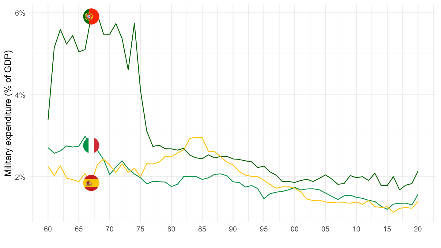
MS.MIL.XPND.GD.ZS |>
  filter(iso2c %in% c("DE", "CH", "KR", "JP")) |>
  left_join(tibble(iso2c = c("DE", "CH", "KR", "JP"),
                   Iso2c = c("Germany", "Switzerland", "South Korea", "Japan")),
            by = "iso2c") |>
  year_to_date() |>
  add_flag_color("Iso2c") |>
  mutate(value = value/100) |>
  ggplot() + geom_line(aes(x = date, y = value, color = color)) +
  xlab("") + ylab("Military expenditure (% of GDP)") +
  theme_minimal() + scale_color_identity() + add_flags +
  scale_x_date(breaks = seq(1950, 2100, 5) |> paste0("-01-01") |> as.Date(),
               labels = date_format("%Y")) +
  scale_y_continuous(breaks = 0.01*seq(-60, 60, 2),
                     labels = scales::percent_format(accuracy = 1))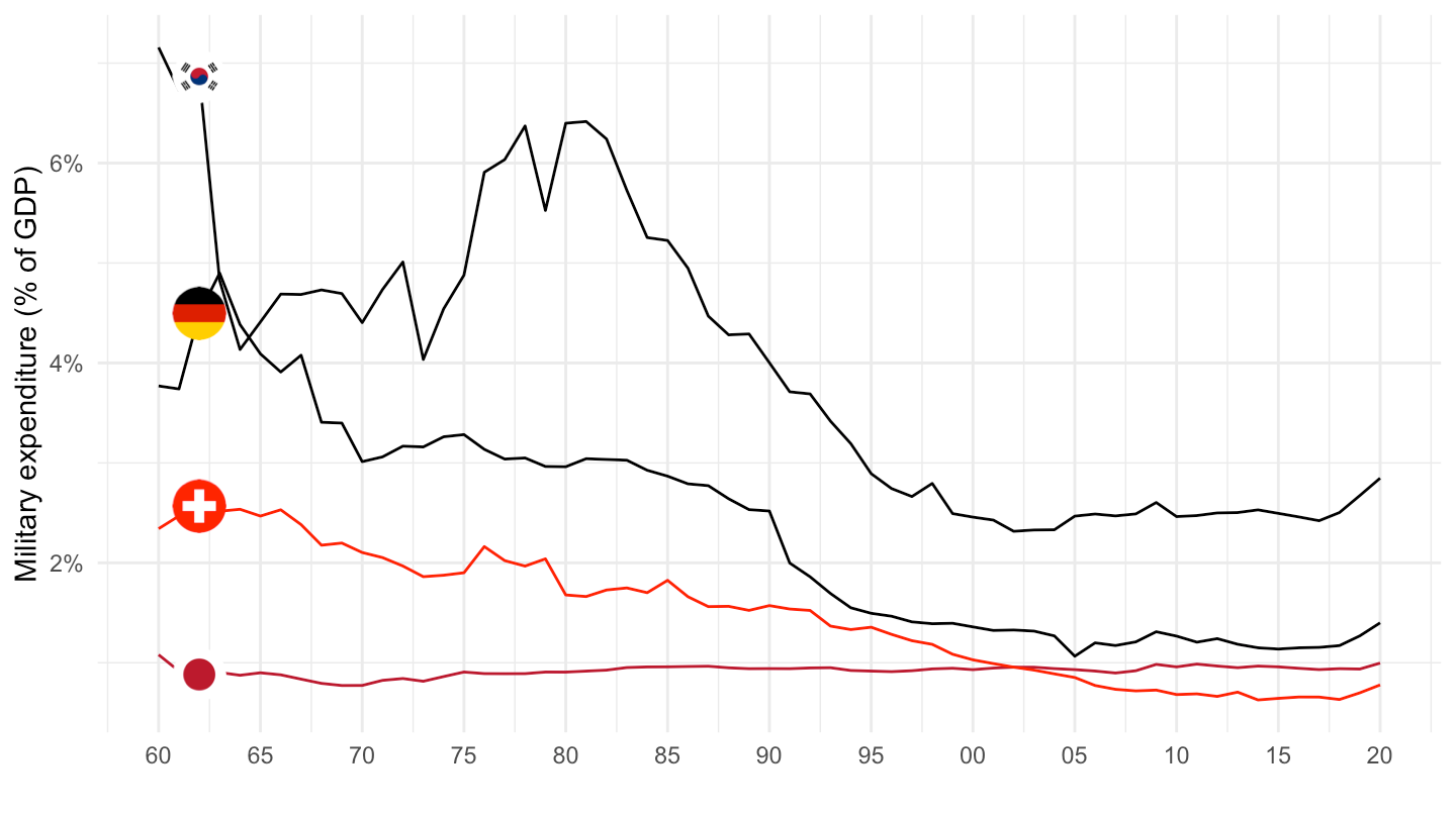
MS.MIL.XPND.GD.ZS |>
  filter(iso2c %in% c("DE", "CH", "KR", "JP")) |>
  left_join(tibble(iso2c = c("DE", "CH", "KR", "JP"),
                   Iso2c = c("Germany", "Switzerland", "South Korea", "Japan")),
            by = "iso2c") |>
  year_to_date() |>
  filter(date >= as.Date("1995-01-01")) |>
  add_flag_color("Iso2c") |>
  mutate(value = value/100) |>
  ggplot() + geom_line(aes(x = date, y = value, color = color)) +
  xlab("") + ylab("Military expenditure (% of GDP)") +
  theme_minimal() + scale_color_identity() + add_flags +
  scale_x_date(breaks = seq(1950, 2100, 5) |> paste0("-01-01") |> as.Date(),
               labels = date_format("%Y")) +
  scale_y_continuous(breaks = 0.01*seq(-60, 60, 2),
                     labels = scales::percent_format(accuracy = 1))
MS.MIL.XPND.GD.ZS |>
  filter(iso2c %in% c("IT", "PT", "ES", "GR", "FR")) |>
  left_join(iso2c, by = "iso2c") |>
  year_to_date() |>
  ggplot() +
  geom_line(aes(x = date, y = value/100, color = Iso2c)) +
  theme_minimal() +
  scale_color_manual(values = c("#002395", "#0D5EAF", "#009246", "#FF0000", "#FFC400")) +
  theme(legend.title = element_blank(),
        legend.position = c(0.2, 0.2)) +
  scale_x_date(breaks = seq(1950, 2100, 5) |> paste0("-01-01") |> as.Date(),
               labels = date_format("%Y")) +
  geom_image(data = . %>%
               filter(date == as.Date("2007-01-01")) %>%
               mutate(image = paste0("../../icon/flag/", str_to_lower(gsub(" ", "-", Iso2c)), ".png")),
             aes(x = date, y = value/100, image = image), asp = 1.5) +
  scale_y_continuous(breaks = 0.01*seq(-60, 60, 2),
                     labels = scales::percent_format(accuracy = 1)) +
  xlab("") + ylab("Military expenditure (% of GDP)")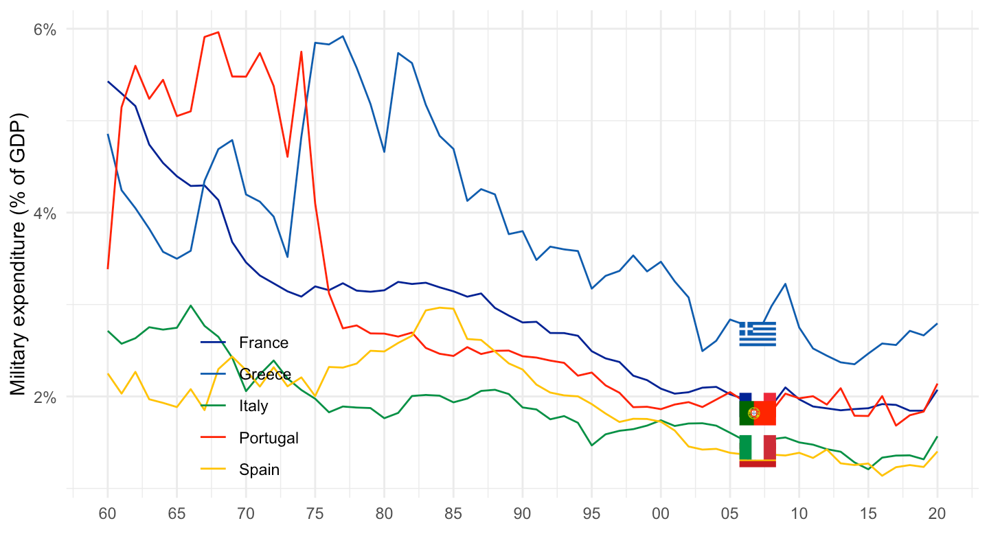
MS.MIL.XPND.GD.ZS |>
  filter(iso2c %in% c("IT", "PT", "ES", "GR", "FR")) |>
  left_join(iso2c, by = "iso2c") |>
  year_to_date() |>
  filter(date >= as.Date("1995-01-01")) |>
  ggplot() +
  geom_line(aes(x = date, y = value/100, color = Iso2c)) +
  theme_minimal() +
  scale_color_manual(values = c("#002395", "#0D5EAF", "#009246", "#FF0000", "#FFC400")) +
  theme(legend.position = "none") +
  scale_x_date(breaks = seq(1950, 2100, 5) |> paste0("-01-01") |> as.Date(),
               labels = date_format("%Y")) +
  geom_image(data = . %>%
               filter(date == as.Date("2016-01-01")) %>%
               mutate(image = paste0("../../icon/flag/", str_to_lower(gsub(" ", "-", Iso2c)), ".png")),
             aes(x = date, y = value/100, image = image), asp = 1.5) +
  scale_y_continuous(breaks = 0.01*seq(-60, 60, 2),
                     labels = scales::percent_format(accuracy = 1)) +
  xlab("") + ylab("Military expenditure (% of GDP)")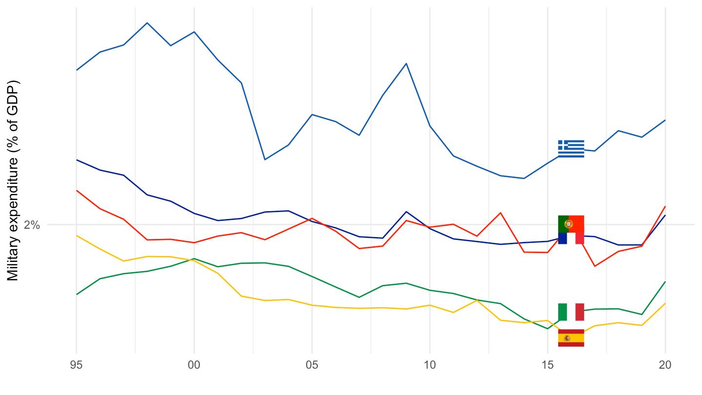
MS.MIL.XPND.GD.ZS |>
  filter(iso2c %in% c("US", "GB")) |>
  left_join(iso2c, by = "iso2c") |>
  year_to_date() |>
  add_flag_color("Iso2c") |>
  mutate(value = value/100) |>
  ggplot() + geom_line(aes(x = date, y = value, color = color)) +
  xlab("") + ylab("Military expenditure (% of GDP)") +
  theme_minimal() + scale_color_identity() + add_flags +
  scale_x_date(breaks = seq(1950, 2100, 5) |> paste0("-01-01") |> as.Date(),
               labels = date_format("%Y")) +
  scale_y_continuous(breaks = 0.01*seq(-60, 60, 2),
                     labels = scales::percent_format(accuracy = 1))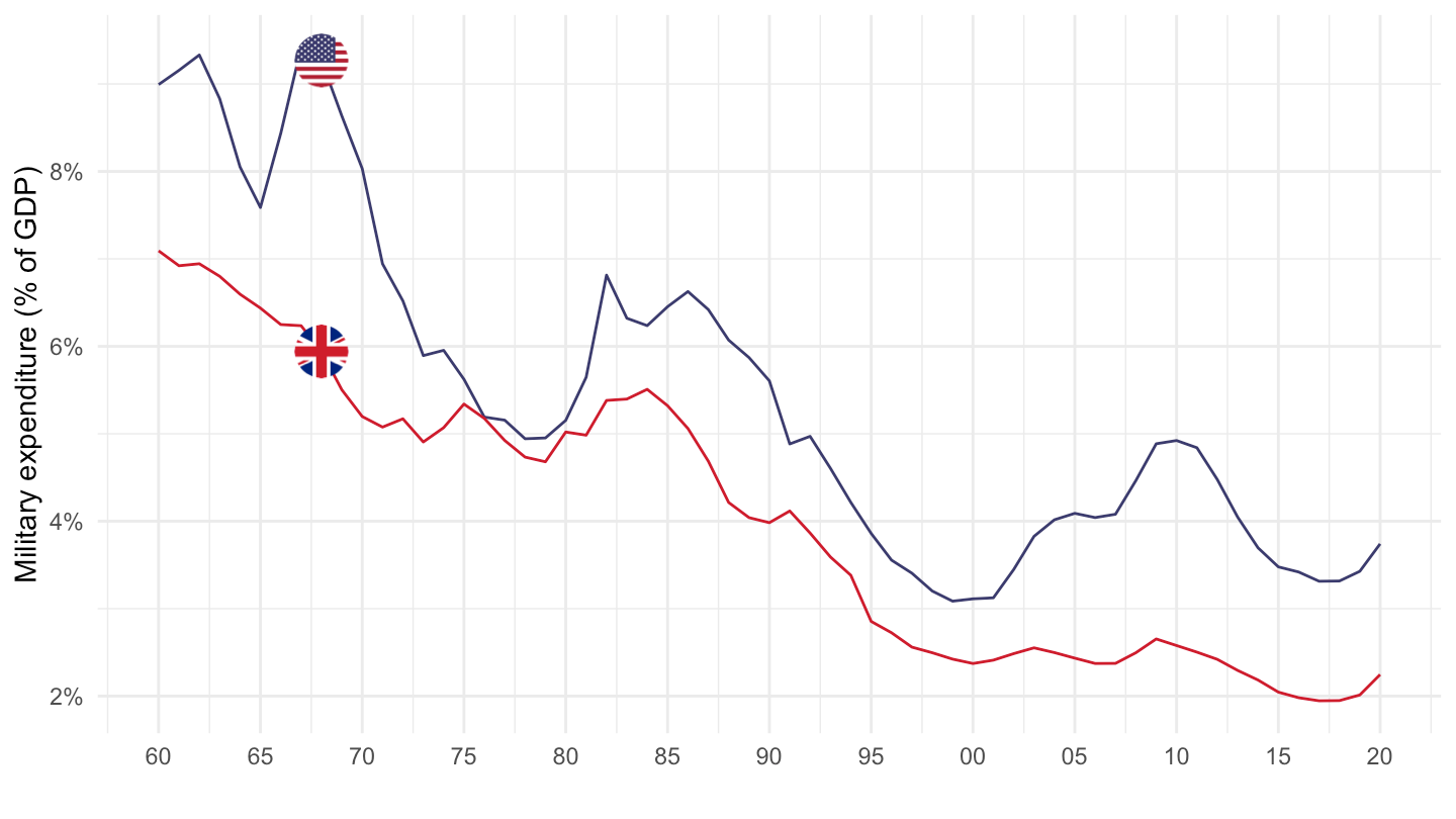
MS.MIL.XPND.GD.ZS |>
  filter(iso2c %in% c("AR", "CL", "VE")) |>
  left_join(tibble(iso2c = c("AR", "CL", "VE"),
                   Iso2c = c("Argentina", "Chile", "Venezuela")),
            by = "iso2c") |>
  year_to_date() |>
  add_flag_color("Iso2c") |>
  mutate(value = value/100) |>
  ggplot() + geom_line(aes(x = date, y = value, color = color)) +
  xlab("") + ylab("Military expenditure (% of GDP)") +
  theme_minimal() + scale_color_identity() + add_flags +
  scale_x_date(breaks = seq(1950, 2100, 5) |> paste0("-01-01") |> as.Date(),
               labels = date_format("%Y")) +
  scale_y_continuous(breaks = 0.01*seq(-60, 60, 2),
                     labels = scales::percent_format(accuracy = 1))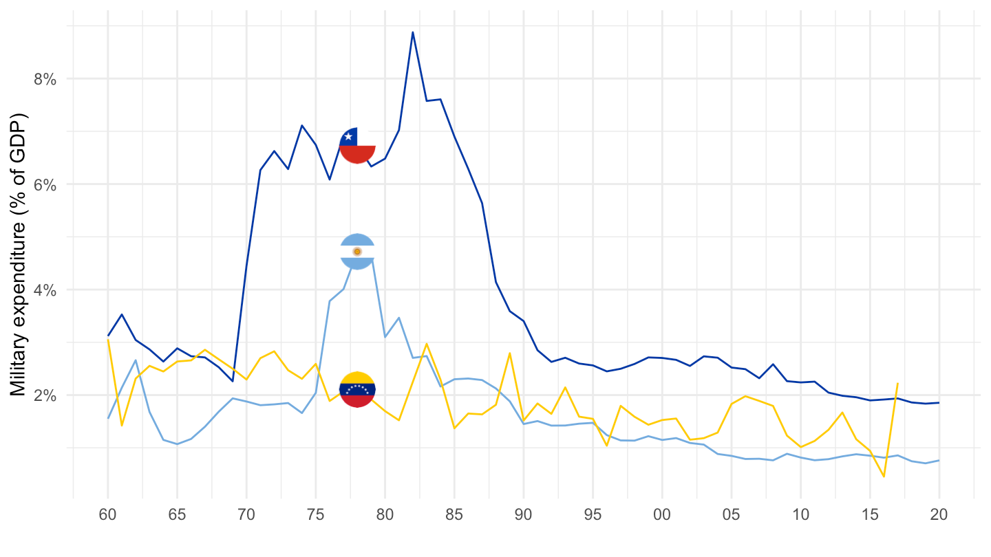
MS.MIL.XPND.GD.ZS |>
  filter(iso2c %in% c("GR", "HK", "MX")) |>
  left_join(iso2c, by = "iso2c") |>
  mutate(Iso2c = ifelse(iso2c == "HK", "Hong Kong", Iso2c)) |>
  year_to_date() |>
  add_flag_color("Iso2c") |>
  mutate(value = value/100) |>
  ggplot() + geom_line(aes(x = date, y = value, color = color)) +
  xlab("") + ylab("Military expenditure (% of GDP)") +
  theme_minimal() + scale_color_identity() + add_flags +
  scale_x_date(breaks = seq(1950, 2100, 5) |> paste0("-01-01") |> as.Date(),
               labels = date_format("%Y")) +
  scale_y_continuous(breaks = 0.01*seq(-60, 60, 2),
                     labels = scales::percent_format(accuracy = 1))