Total greenhouse gas emissions (kt of CO2 equivalent) - EN.ATM.GHGT.KT.CE

Data - WDI

Author

François Geerolf

Info

Last observation: 2020 (N = 7,408)

First observation: 1990 (N = 7,408)

Last data update: 24 jul 2026, 15:30. Last compile: 13 aoû 2026, 23:05

Info

DOWNLOAD_TIME

Code

tibble(DOWNLOAD_TIME = as.Date(file.info("~/iCloud/website/data/wdi/value.RData")$mtime)) |>
  print_table_conditional()

DOWNLOAD_TIME
NA

Last

Code

EN.ATM.GHGT.KT.CE |>
  group_by(year) |>
  summarise(Nobs = n()) |>
  arrange(desc(year)) |>
  head(1) |>
  print_table_conditional()

year	Nobs
2020	239

1960, 2018

All

Code

EN.ATM.GHGT.KT.CE |>
  left_join(iso2c, by = "iso2c") |>
  group_by(iso2c, Iso2c) |>
  mutate(value = round(value, 2)) |>
  summarise(Nobs = n(),
            `Year 1` = first(year),
            `CO2 emissions (kt) 1` = first(value),
            `Year 2` = last(year),
            `CO2 emissions (kt) 2` = last(value)) |>
  arrange(-`CO2 emissions (kt) 2`) |>
  mutate(Flag = gsub(" ", "-", str_to_lower(Iso2c)),
         Flag = paste0('<img src="../../bib/flags/vsmall/', Flag, '.png" alt="Flag">')) |>
  select(Flag, everything()) %>%
  {if (is_html_output()) datatable(., filter = 'top', rownames = F, escape = F) else .}

China, E.U., U.S.

Part

Code

EN.ATM.GHGT.KT.CE |>
  right_join(iso2c, by = "iso2c") |>
  filter(iso2c %in% c("1W", "US", "CN", "EU")) |>
  group_by(year) |>
  mutate(value = value/value[iso2c == "1W"]) |>
  year_to_date() |>
  filter(!(iso2c == "1W")) |>
  mutate(Iso2c = ifelse(iso2c == "EU", "Europe", Iso2c)) |>
  left_join(colors, by = c("Iso2c" = "country")) |>
  mutate(color = ifelse(iso2c == "US", color2, color)) |>
  ggplot() + theme_minimal() + scale_color_identity() +
  geom_line(aes(x = date, y = value, color = color)) +
  add_flags +
  scale_x_date(breaks = seq(1950, 2100, 5) |> paste0("-01-01") |> as.Date(),
               labels = date_format("%Y")) +
  scale_y_continuous(breaks = 0.01*seq(0, 70, 5),
                     labels = scales::percent_format(accuracy = 1),
                     limits = 0.01*c(0, 35)) + 
  xlab("") + ylab("Total greenhouse gas emissions (kt of CO2 equivalent)")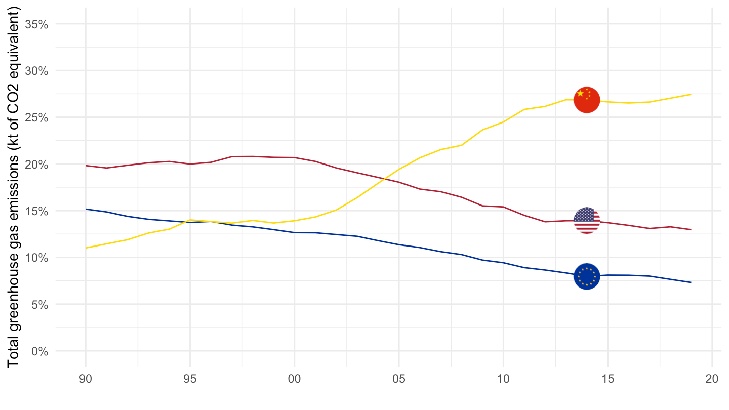

Valeur

Code

EN.ATM.GHGT.KT.CE |>
  right_join(iso2c, by = "iso2c") |>
  filter(iso2c %in% c("US", "CN", "EU")) |>
  mutate(value = value / 1000) |>
  year_to_date() |>
  mutate(Iso2c = ifelse(iso2c == "EU", "Europe", Iso2c)) |>
  left_join(colors, by = c("Iso2c" = "country")) |>
  mutate(color = ifelse(iso2c == "US", color2, color)) |>
  ggplot() + theme_minimal() + scale_color_identity() +
  geom_line(aes(x = date, y = value, color = color)) +
  add_flags +
  scale_x_date(breaks = seq(1950, 2100, 5) |> paste0("-01-01") |> as.Date(),
               labels = date_format("%Y")) +
  xlab("") + ylab("Emissions de CO2 en Mt") +
  scale_y_continuous(breaks = seq(0, 100000, 1000),
                     labels = dollar_format(prefix = "", suffix = " Mt"))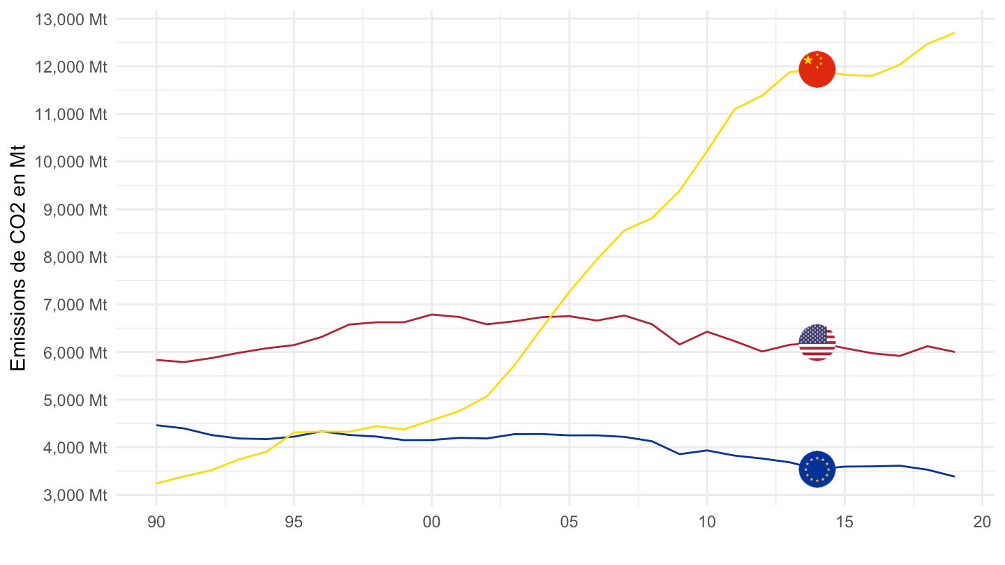

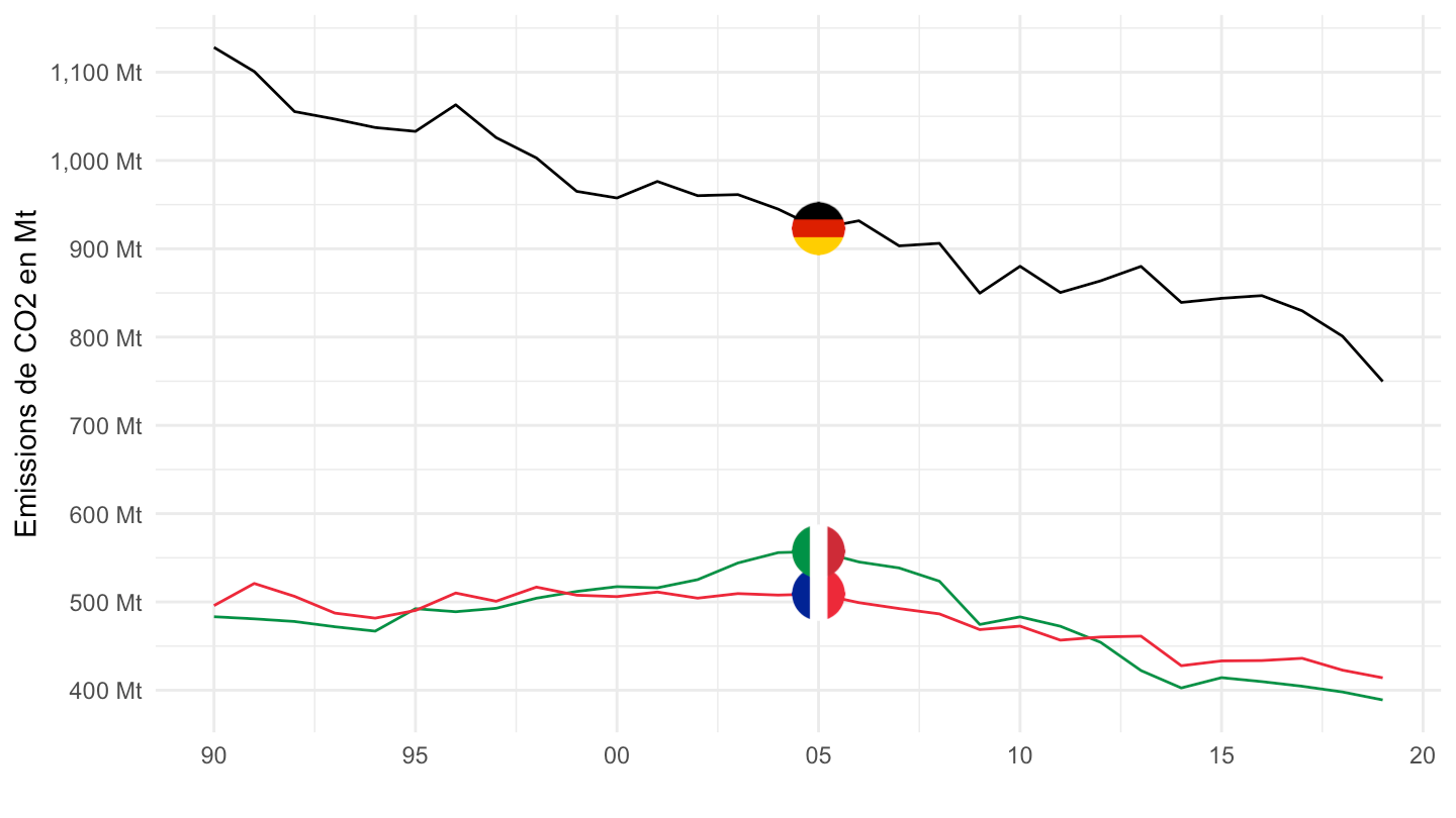
France, Germany, Italy

Part

Code

EN.ATM.GHGT.KT.CE |>
  right_join(iso2c, by = "iso2c") |>
  filter(iso2c %in% c("1W", "IT", "FR", "DE")) |>
  group_by(year) |>
  mutate(value = value/value[iso2c == "1W"]) |>
  year_to_date() |>
  filter(!(iso2c == "1W")) |>
  left_join(colors, by = c("Iso2c" = "country")) |>
  mutate(color = ifelse(iso2c == "US", color2, color)) |>
  ggplot() + theme_minimal() + scale_color_identity() +
  geom_line(aes(x = date, y = value, color = color)) +
  add_flags +
  scale_x_date(breaks = seq(1950, 2100, 5) |> paste0("-01-01") |> as.Date(),
               labels = date_format("%Y")) +
  scale_y_continuous(breaks = 0.01*seq(0, 70, 1),
                     labels = scales::percent_format(accuracy = 1),
                     limits = 0.01*c(0, 5)) + 
  xlab("") + ylab("Total greenhouse gas emissions (kt of CO2 equivalent)")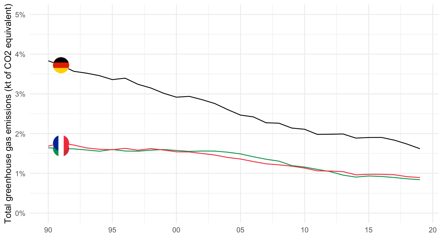

Valeur

Code

EN.ATM.GHGT.KT.CE |>
  filter(iso2c %in% c("IT", "FR", "DE")) |>
  left_join(iso2c, by = "iso2c") |>
  mutate(value = value / 1000) |>
  year_to_date() |>
  mutate(Iso2c = ifelse(iso2c == "EU", "Europe", Iso2c)) |>
  left_join(colors, by = c("Iso2c" = "country")) |>
  mutate(color = ifelse(iso2c == "US", color2, color)) |>
  ggplot() + theme_minimal() + scale_color_identity() +
  geom_line(aes(x = date, y = value, color = color)) +
  add_flags +
  scale_x_date(breaks = seq(1950, 2100, 5) |> paste0("-01-01") |> as.Date(),
               labels = date_format("%Y")) +
  xlab("") + ylab("Emissions de CO2 en Mt") +
  scale_y_continuous(breaks = seq(0, 100000, 100),
                     labels = dollar_format(prefix = "", suffix = " Mt"))