Code
MIm_var$subject %>%
print_table_conditional| subject | Subject |
|---|---|
| E | Employee |
| EP | Employed person |
| LB | Labour force |
| NILF | Not in labour force |
| UE | Unemployed person |
| UR | Unemployment rate |
Data - Statjp
MIm_var$subject %>%
print_table_conditional| subject | Subject |
|---|---|
| E | Employee |
| EP | Employed person |
| LB | Labour force |
| NILF | Not in labour force |
| UE | Unemployed person |
| UR | Unemployment rate |
MIm_var$seasonally_adjusted %>%
print_table_conditional| seasonally_adjusted | Seasonally adjusted |
|---|---|
| NSA | not seasonally adjusted |
| SA | seasonally adjusted |
MIm_var$sex %>%
print_table_conditional| sex | Sex |
|---|---|
| B | Both sexes |
| F | Female |
| M | Male |
MIm_var$unit %>%
print_table_conditional| unit | Unit |
|---|---|
| PCT | Percent |
| TTP | Ten thousand persons |
MIm %>%
  group_by(series_code, series_name) %>%
  summarise(Nobs = n()) %>%
print_table_conditionalMIm %>%
filter(subject == "UR",
seasonally_adjusted == "SA") %>%
ggplot(.) + geom_line(aes(x = period, y = value/100, color = Sex)) +
theme_minimal() + xlab("") + ylab("") +
scale_x_date(breaks = seq(1940, 2020, 5) %>% paste0("-01-01") %>% as.Date,
labels = date_format("%y")) +
scale_y_continuous(breaks = 0.01*seq(0, 200, 1),
labels = percent_format(acc = 1)) +
scale_color_manual(values = viridis(4)[1:3]) +
theme(legend.position = c(0.2, 0.8),
legend.title = element_blank())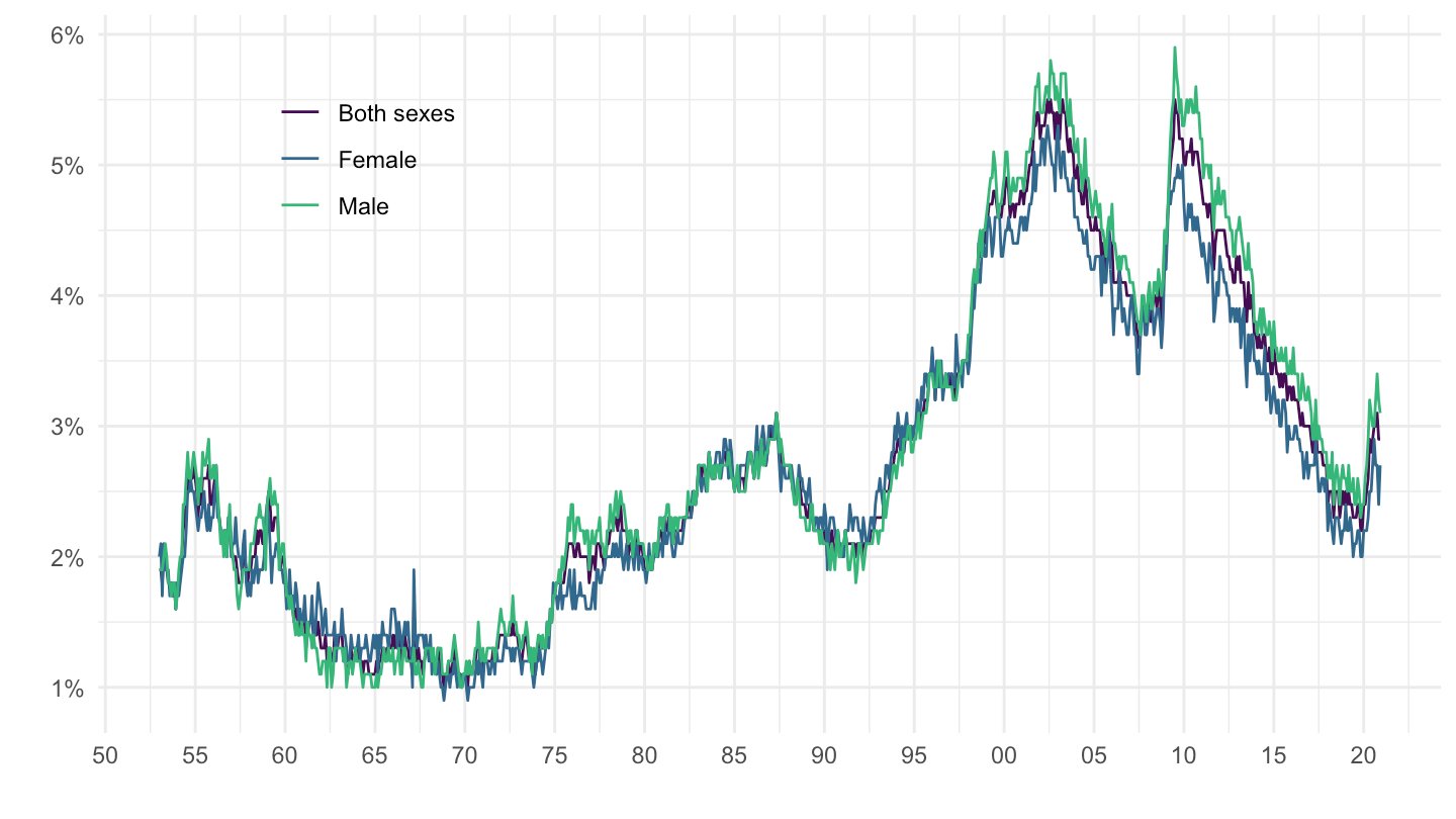
MIm %>%
  filter(subject == "UR",
         seasonally_adjusted == "SA",
         period >= as.Date("1985-01-01"),
         period <= as.Date("2000-01-01")) %>%
  ggplot(.) + geom_line(aes(x = period, y = value/100, color = Sex)) +
  theme_minimal() + xlab("") + ylab("") +
  scale_x_date(breaks = seq(1940, 2020, 1) %>% paste0("-01-01") %>% as.Date,
               labels = date_format("%y")) +
  scale_y_continuous(breaks = 0.01*seq(0, 200, 1),
                labels = percent_format(acc = 1)) +
  scale_color_manual(values = viridis(4)[1:3]) +
  theme(legend.position = c(0.2, 0.8),
        legend.title = element_blank())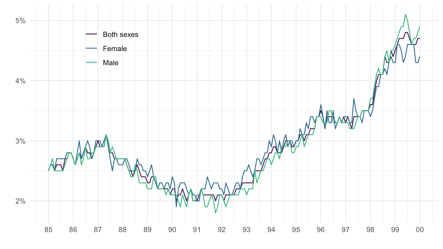
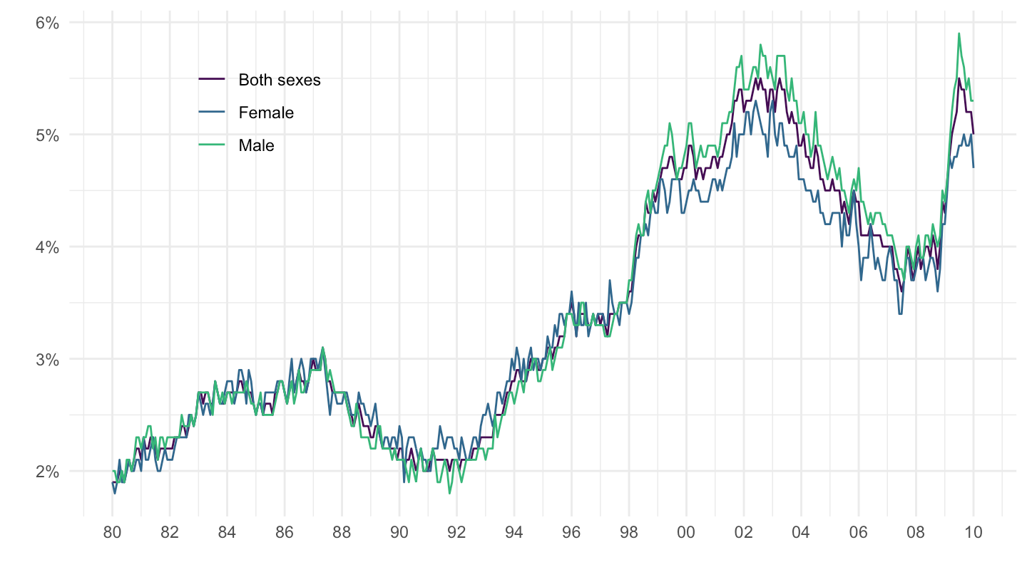
MIm %>%
  filter(subject == "UR",
         seasonally_adjusted == "SA",
         period >= as.Date("1980-01-01"),
         period <= as.Date("2010-01-01")) %>%
  ggplot(.) + geom_line(aes(x = period, y = value/100, color = Sex)) +
  theme_minimal() + xlab("") + ylab("") +
  scale_x_date(breaks = seq(1940, 2020, 2) %>% paste0("-01-01") %>% as.Date,
               labels = date_format("%y")) +
  scale_y_continuous(breaks = 0.01*seq(0, 200, 1),
                labels = percent_format(acc = 1)) +
  scale_color_manual(values = viridis(4)[1:3]) +
  theme(legend.position = c(0.2, 0.8),
        legend.title = element_blank())