ULC_QUA %>%
filter(SUBJECT == "ULQBBU99",
SECTOR == "01",
MEASURE == "IXOBTE",
FREQUENCY == "Q",
LOCATION %in% c("FRA", "DEU", "ITA", "GRC", "ESP")) %>%
left_join(ULC_QUA_var$LOCATION %>%
setNames(c("LOCATION", "Location")), by = "LOCATION") %>%
quarter_to_date %>%
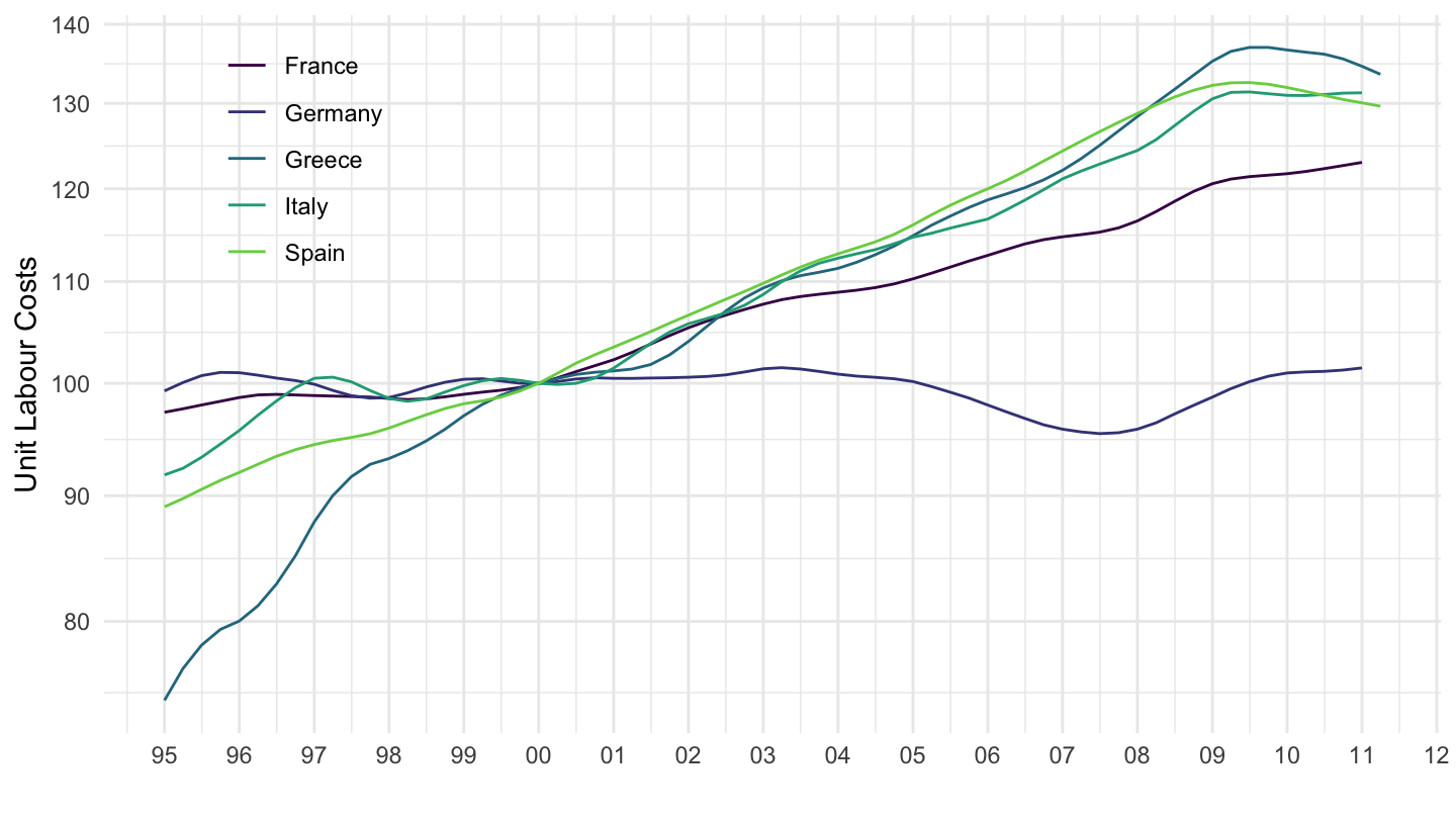
filter(date >= as.Date("1995-01-01")) %>%
group_by(Location) %>%
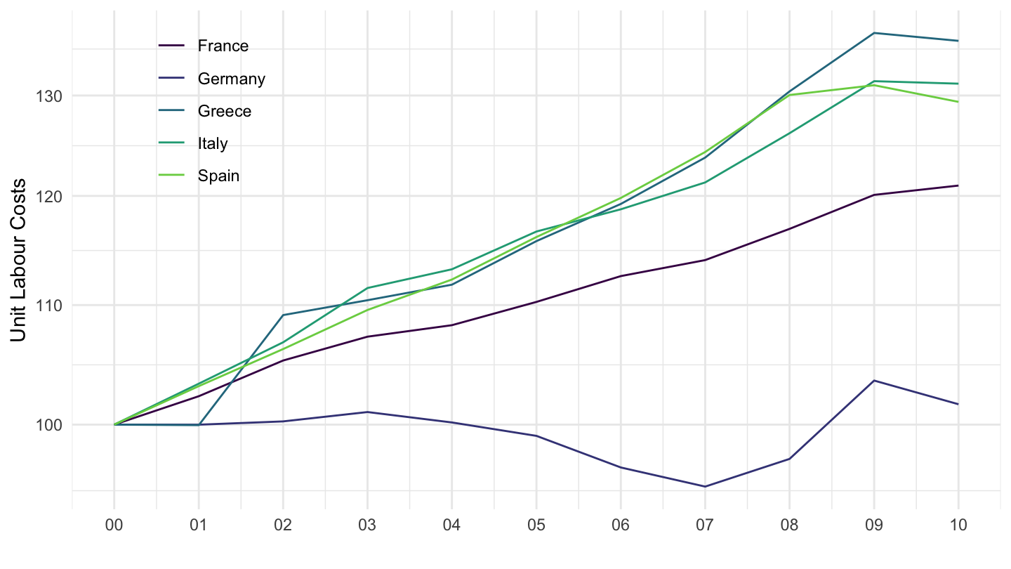
mutate(obsValue = 100*obsValue / obsValue[date == as.Date("2000-01-01")]) %>%
ggplot() + theme_minimal() + ylab("Unit Labour Costs") + xlab("") +
geom_line(aes(x = date, y = obsValue, color = Location)) +
scale_color_manual(values = viridis(6)[1:5]) +
theme(legend.position = c(0.15, 0.8),
legend.title = element_blank()) +
scale_x_date(breaks = seq(1920, 2025, 1) %>% paste0("-01-01") %>% as.Date,
labels = date_format("%y")) +
scale_y_log10(breaks = seq(0, 200, 10))